1. Problem Solving as Search

2. Problem Types Deterministic, fully observable  single-state problem Non-observable  conformant problem Nondeterministic and/or partially observable  contingency problem Unknown state space  exploration problem

3. Consider this problem Five missionaries and five cannibals Want to cross a river using one canoe. Canoe can hold up to three people. Can never be more cannibals than missionaries on either side of the river. Aim: To get all safely across the river without any missionaries being eaten. States?? Actions?? Goal test?? Path cost??

4. Single-State Problem Formulation A problem is defined by four items: 1.initial state 2.successor function (which actually defines all reachable states) 3.goal test 4.path cost (additive) e.g., sum of distances, number of actions executed, etc. C(x,a,y) is the step cost, assumed to be  0

5. Problem Representation : Cannibals and Missionaries Initial State –We can show number of cannibals, missionaries and canoes on each side of the river. –Start state is therefore: [5,5,1,0,0,0]

6. Problem Representation : Cannibals and Missionaries Initial State –However, since the system is closed, we only need to represent one side of the river, as we can deduce the other side. –We will represent the starting side of the river, and omit the ending side. –So start state is: [5,5,1]

7. Problem Representation : Cannibals and Missionaries Goal State(s) –[0,0,0] –TECHNICALLY also [0,0,1]

8. Problem Representation : Cannibals and Missionaries Successor Function (9 actions) 1.Move one missionary. 2.Move one cannibal. 3.Move two missionaries. 4.Move two cannibals. 5.Move three missionaries. 6.Move three cannibals. 7.Move one missionary and one cannibal. 8.Move one missionary and two cannibals. 9.Move two missionaries and one cannibal.

9. Problem Representation : Cannibals and Missionaries Successor Function (9 actions) 1.Move one missionary. 2.Move one cannibal. 3.Move two missionaries. 4.Move two cannibals. 5.Move three missionaries. 6.Move three cannibals. 7.Move one missionary and one cannibal. 8.Move one missionary and two cannibals. 9.Move two missionaries and one cannibal.

10. Problem Representation : Cannibals and Missionaries Successor Function –To be a little more mathematical/computer like, we want to represent this in a true successor function format… S(state)  state 1.Move one cannibal across the river. S([x,y,1])  [x-1,y,0] S([x,y,0])  [x+1,y,1] [Note, this is a slight simplification. We also require, 0  x, y, [x+1 or x-1]  5 ]

11. Problem Representation : Cannibals and Missionaries Successor Function S([x,y,0])  [x+1,y,1] //1 missionary S([x,y,1])  [x-1,y,0] … S([x,y,0])  [x+2,y,1] //2 missionaries S([x,y,1])  [x-2,y,0] … S([x,y,0])  [x+1,y+1,1] // 1 of each S([x,y,1])  [x-1,y-1,0]

12. Problem Representation : Cannibals and Missionaries Path Cost –One unit per trip across the river.

13. Implementation: General Tree Search

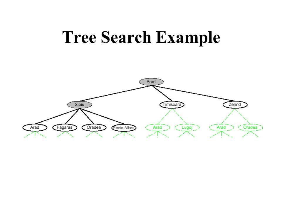
14. Tree Search Example

16. Uninformed Search Strategies Uninformed strategies use only information available in the problem definition –Breadth-first search –Uniform-cost search –Depth-first search –Depth-limited search –Iterative deepening search

17. Uninformed Search Strategies Uninformed strategies use only information available in the problem definition –Breadth-first search –Uniform-cost search –Depth-first search –Depth-limited search –Iterative deepening search

18. Breadth-First Search Expanding shallowest unexpanded node Implementation fringe is a FIFO queue, i.e., new successors go at end

19. Breadth-First Search Expanding shallowest unexpanded node Implementation fringe is a FIFO queue, i.e., new successors go at end

20. Breadth-First Search Expanding shallowest unexpanded node Implementation fringe is a FIFO queue, i.e., new successors go at end

21. Breadth-First Search Expanding shallowest unexpanded node Implementation fringe is a FIFO queue, i.e., new successors go at end

22. Depth-First Search Expand deepest unexpanded node Implementation: fringe = LIFO queue, I.e., put successors at front

23. Depth-First Search Expand deepest unexpanded node Implementation: fringe = LIFO queue, I.e., put successors at front

24. Depth-First Search Expand deepest unexpanded node Implementation: fringe = LIFO queue, I.e., put successors at front

25. Depth-First Search Expand deepest unexpanded node Implementation: fringe = LIFO queue, I.e., put successors at front

26. Depth-First Search Expand deepest unexpanded node Implementation: fringe = LIFO queue, I.e., put successors at front

27. Depth-First Search Expand deepest unexpanded node Implementation: fringe = LIFO queue, I.e., put successors at front

28. Depth-First Search Expand deepest unexpanded node Implementation: fringe = LIFO queue, I.e., put successors at front

29. Depth-First Search Expand deepest unexpanded node Implementation: fringe = LIFO queue, I.e., put successors at front

30. Depth-First Search Expand deepest unexpanded node Implementation: fringe = LIFO queue, I.e., put successors at front

31. Depth-First Search Expand deepest unexpanded node Implementation: fringe = LIFO queue, I.e., put successors at front

32. Depth-First Search Expand deepest unexpanded node Implementation: fringe = LIFO queue, I.e., put successors at front

33. Depth-First Search Expand deepest unexpanded node Implementation: fringe = LIFO queue, I.e., put successors at front

34. Search Strategies A strategy is defined by picking the order of node expansion Strategies are evaluated along the following dimensions: completeness – does it always find a solution if one exists? time complexity – number of nodes generated/expanded space complexity – maximum number of nodes in memory optimality – does it always find a least-cost solution

35. This is how far we got

36. Search Strategies Time and space complexity are measured in terms of b – maximum branching factor of the search tree d – depth of the least-cost solution m – maximum depth of the state space (may be infinite)

37. Properties of Depth-first Search Complete??

38. Properties of Depth-first Search Complete?? No: fails in infinite-depth spaces, spaces with loops Modify to avoid repeated states along path  complete in finite spaces Time??

39. Properties of Depth-first Search Complete?? No: fails in infinite-depth spaces, spaces with loops Modify to avoid repeated states along path  complete in finite spaces Time?? O(b m ): terrible if m is much larger than d but if solutions are dense, may be much faster than breadth-first Space??

40. Properties of Depth-first Search Complete?? No: fails in infinite-depth spaces, spaces with loops Modify to avoid repeated states along path  complete in finite spaces Time?? O(b m ): terrible if m is much larger than d but if solutions are dense, may be much faster than breadth-first Space?? O(bm), I.e., linear space! Optimal??

41. Properties of Depth-first Search Complete?? No: fails in infinite-depth spaces, spaces with loops Modify to avoid repeated states along path  complete in finite spaces Time?? O(b m ): terrible if m is much larger than d but if solutions are dense, may be much faster than breadth-first Space?? O(bm), I.e., linear space! Optimal?? No.

42. Properties of Breadth-First Search Complete??

43. Properties of Breadth-First Search Complete?? Yes (if b is finite) Time??

44. Properties of Breadth-First Search Complete?? Yes (if b is finite) Time?? 1 + b + b 2 + b 3 + … + b d + b(b d – 1) = O( b d+1 ), ie, exp. in d Space??

45. Properties of Breadth-First Search Complete?? Yes (if b is finite) Time?? 1 + b + b 2 + b 3 + … + b d + b(b d – 1) = O( b d+1 ), ie, exp. in d Space?? O( b d+1 ) (keep every node in memory) Optimal??

46. Properties of Breadth-First Search Complete?? Yes (if b is finite) Time?? 1 + b + b 2 + b 3 + … + b d + b(b d – 1) = O( b d+1 ), ie, exp. in d Space?? O( b d+1 ) (keep every node in memory) Optimal?? Yes (if cost = 1 per step); not optimal in general Space is the big problem: can easily generate nodes at 10MB/sec, so 24hours = 860GB.

47. Implementation: General Tree Search