1. Feature extraction: Corners and blobs

2. Why extract features? Motivation: panorama stitching We have two images – how do we combine them?

3. Why extract features? Motivation: panorama stitching We have two images – how do we combine them? Step 1: extract features Step 2: match features

4. Why extract features? Motivation: panorama stitching We have two images – how do we combine them? Step 1: extract features Step 2: match features Step 3: align images

5. Characteristics of good features Repeatability The same feature can be found in several images despite geometric and photometric transformations Saliency Each feature has a distinctive description Compactness and efficiency Many fewer features than image pixels Locality A feature occupies a relatively small area of the image; robust to clutter and occlusion

6. Applications Feature points are used for: Motion tracking Image alignment 3D reconstruction Object recognition Indexing and database retrieval Robot navigation

7. Finding Corners Key property: in the region around a corner, image gradient has two or more dominant directions Corners are repeatable and distinctive C.Harris and M.Stephens. "A Combined Corner and Edge Detector.“ Proceedings of the 4th Alvey Vision Conference: pages 147--151. "A Combined Corner and Edge Detector.“

8. Corner Detection: Basic Idea We should easily recognize the point by looking through a small window Shifting a window in any direction should give a large change in intensity “edge”: no change along the edge direction “corner”: significant change in all directions “flat” region: no change in all directions Source: A. Efros

9. Corner Detection: Mathematics Change in appearance for the shift [u,v]: Intensity Shifted intensity Window function or Window function w(x,y) = Gaussian1 in window, 0 outside Source: R. Szeliski

10. Corner Detection: Mathematics Change in appearance for the shift [u,v]: I(x, y) E(u, v) E(0,0) E(3,2)

11. Corner Detection: Mathematics Change in appearance for the shift [u,v]: Second-order Taylor expansion of E(u,v) about (0,0) (local quadratic approximation): We want to find out how this function behaves for small shifts

12. Corner Detection: Mathematics Second-order Taylor expansion of E(u,v) about (0,0):

13. Corner Detection: Mathematics Second-order Taylor expansion of E(u,v) about (0,0):

14. Corner Detection: Mathematics Second-order Taylor expansion of E(u,v) about (0,0):

15. Corner Detection: Mathematics The quadratic approximation simplifies to where M is a second moment matrix computed from image derivatives: M

16. The surface E(u,v) is locally approximated by a quadratic form. Let’s try to understand its shape. Interpreting the second moment matrix

17. First, consider the axis-aligned case (gradients are either horizontal or vertical) If either λ is close to 0, then this is not a corner, so look for locations where both are large. Interpreting the second moment matrix

18. Consider a horizontal “slice” of E(u, v): Interpreting the second moment matrix This is the equation of an ellipse.

19. Consider a horizontal “slice” of E(u, v): Interpreting the second moment matrix This is the equation of an ellipse. The axis lengths of the ellipse are determined by the eigenvalues and the orientation is determined by R direction of the slowest change direction of the fastest change ( max ) -1/2 ( min ) -1/2 Diagonalization of M:

20. Visualization of second moment matrices

22. Interpreting the eigenvalues 1 2 “Corner” 1 and 2 are large, 1 ~ 2 ; E increases in all directions 1 and 2 are small; E is almost constant in all directions “Edge” 1 >> 2 “Edge” 2 >> 1 “Flat” region Classification of image points using eigenvalues of M:

23. Corner response function “Corner” R > 0 “Edge” R < 0 “Flat” region |R| small α : constant (0.04 to 0.06)

24. Harris detector: Steps 1.Compute Gaussian derivatives at each pixel 2.Compute second moment matrix M in a Gaussian window around each pixel 3.Compute corner response function R 4.Threshold R 5.Find local maxima of response function (nonmaximum suppression) C.Harris and M.Stephens. "A Combined Corner and Edge Detector.“ Proceedings of the 4th Alvey Vision Conference: pages 147—151, 1988. "A Combined Corner and Edge Detector.“

25. Harris Detector: Steps

26. Compute corner response R

27. Harris Detector: Steps Find points with large corner response: R>threshold

28. Harris Detector: Steps Take only the points of local maxima of R

29. Harris Detector: Steps

30. Invariance and covariance We want features to be invariant to photometric transformations and covariant to geometric transformations Invariance: image is transformed and features do not change Covariance: if we have two transformed versions of the same image, features should be detected in corresponding locations

31. Models of Image Change Photometric Affine intensity change ( I  a I + b) Geometric Rotation Scale Affine valid for: orthographic camera, locally planar object

32. Affine intensity change Only derivatives are used => invariance to intensity shift I  I + b Intensity scale: I  a I R x (image coordinate) threshold R x (image coordinate) Partially invariant to affine intensity change

33. Image rotation Ellipse rotates but its shape (i.e. eigenvalues) remains the same Corner response R is invariant w.r.t. rotation and corner location is covariant

34. Scaling All points will be classified as edges Corner Not invariant to scaling

35. Achieving scale covariance Goal: independently detect corresponding regions in scaled versions of the same image Need scale selection mechanism for finding characteristic region size that is covariant with the image transformation

36. Blob detection with scale selection

37. Recall: Edge detection f Source: S. Seitz Edge Derivative of Gaussian Edge = maximum of derivative

38. Edge detection, Take 2 f Edge Second derivative of Gaussian (Laplacian) Edge = zero crossing of second derivative Source: S. Seitz

39. From edges to blobs Edge = ripple Blob = superposition of two ripples Spatial selection: the magnitude of the Laplacian response will achieve a maximum at the center of the blob, provided the scale of the Laplacian is “matched” to the scale of the blob maximum

40. Scale selection We want to find the characteristic scale of the blob by convolving it with Laplacians at several scales and looking for the maximum response However, Laplacian response decays as scale increases: Why does this happen? increasing σ original signal (radius=8)

41. Scale normalization The response of a derivative of Gaussian filter to a perfect step edge decreases as σ increases

42. Scale normalization The response of a derivative of Gaussian filter to a perfect step edge decreases as σ increases To keep response the same (scale-invariant), must multiply Gaussian derivative by σ Laplacian is the second Gaussian derivative, so it must be multiplied by σ 2

43. Effect of scale normalization Scale-normalized Laplacian response Unnormalized Laplacian response Original signal maximum

44. Blob detection in 2D Laplacian of Gaussian: Circularly symmetric operator for blob detection in 2D

45. Blob detection in 2D Laplacian of Gaussian: Circularly symmetric operator for blob detection in 2D Scale-normalized:

46. Scale selection At what scale does the Laplacian achieve a maximum response to a binary circle of radius r? r imageLaplacian

47. Scale selection At what scale does the Laplacian achieve a maximum response to a binary circle of radius r? To get maximum response, the zeros of the Laplacian have to be aligned with the circle The Laplacian is given by (up to scale): Therefore, the maximum response occurs at r image circle Laplacian

48. Characteristic scale We define the characteristic scale of a blob as the scale that produces peak of Laplacian response in the blob center characteristic scale T. Lindeberg (1998). "Feature detection with automatic scale selection." International Journal of Computer Vision 30 (2): pp 77--116."Feature detection with automatic scale selection."

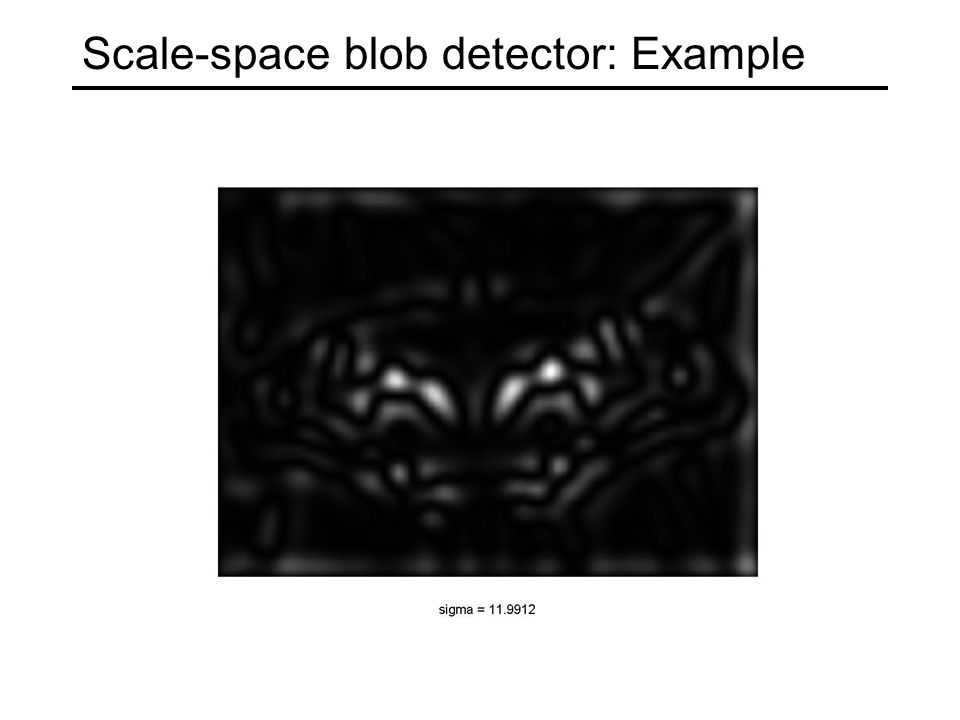
49. Scale-space blob detector 1.Convolve image with scale-normalized Laplacian at several scales 2.Find maxima of squared Laplacian response in scale-space

50. Scale-space blob detector: Example

53. Approximating the Laplacian with a difference of Gaussians: (Laplacian) (Difference of Gaussians) Efficient implementation

54. David G. Lowe. "Distinctive image features from scale-invariant keypoints.” IJCV 60 (2), pp. 91-110, 2004."Distinctive image features from scale-invariant keypoints.”

55. Invariance and covariance properties Laplacian (blob) response is invariant w.r.t. rotation and scaling Blob location is covariant w.r.t. rotation and scaling What about intensity change?

56. Achieving affine covariance direction of the slowest change direction of the fastest change ( max ) -1/2 ( min ) -1/2 Consider the second moment matrix of the window containing the blob: Recall: This ellipse visualizes the “characteristic shape” of the window

57. Affine adaptation example Scale-invariant regions (blobs)

58. Affine adaptation example Affine-adapted blobs

59. Affine adaptation Problem: the second moment “window” determined by weights w(x,y) must match the characteristic shape of the region Solution: iterative approach Use a circular window to compute second moment matrix Perform affine adaptation to find an ellipse-shaped window Recompute second moment matrix using new window and iterate

60. Iterative affine adaptation K. Mikolajczyk and C. Schmid, Scale and Affine invariant interest point detectors, IJCV 60(1):63-86, 2004.Scale and Affine invariant interest point detectors http://www.robots.ox.ac.uk/~vgg/research/affine/

61. Affine covariance Affinely transformed versions of the same neighborhood will give rise to ellipses that are related by the same transformation What to do if we want to compare these image regions? Affine normalization: transform these regions into same-size circles

62. Affine normalization Problem: There is no unique transformation from an ellipse to a unit circle We can rotate or flip a unit circle, and it still stays a unit circle

63. Eliminating rotation ambiguity To assign a unique orientation to circular image windows: Create histogram of local gradient directions in the patch Assign canonical orientation at peak of smoothed histogram 0 2 

64. From covariant regions to invariant features Extract affine regionsNormalize regions Eliminate rotational ambiguity Compute appearance descriptors SIFT (Lowe ’04)

65. Invariance vs. covariance Invariance: features(transform(image)) = features(image) Covariance: features(transform(image)) = transform(features(image)) Covariant detection => invariant description