1. Correlation Forensic Statistics CIS205

2. Introduction Chi-squared shows the strength of relationship between variables when the data is of count form However, many variables measured in a lab are on a continuous scale, such as concentrations of chemicals, time, and most machine responses The term for the strength of the relation between continuous variables is correlation Any continuous variables which have some sort of systematic relationship are said to covary, and any variable which covaries with another is said to be a covariate. A basic tool for the investigation of correlation is the scatterplot. Usually only two variables are plotted, but three can be accommodated.

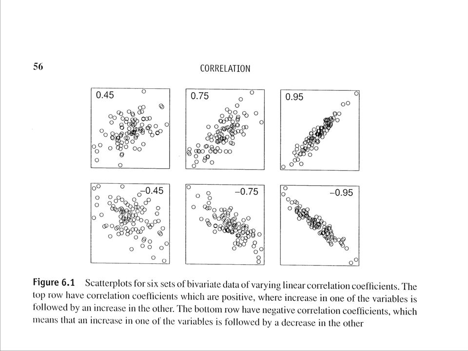
3. Correlation Coefficient A statistical measure of correlation is called the correlation coefficient, which can only take on values between -1 and 1. Both 1 and -1 mean that the variables are absolutely related 1 means that as one variable increases, so does the other -1 means that as one variable increases, the other decreases. 0 means that the variables are unrelated. The strength of relationship is independent of the form of relationship. Most commonly relationships are linear (plotting one variable against another yields a straight line), next most commonly loglinear (a graph of one variable against the logarithm of the other is linear).

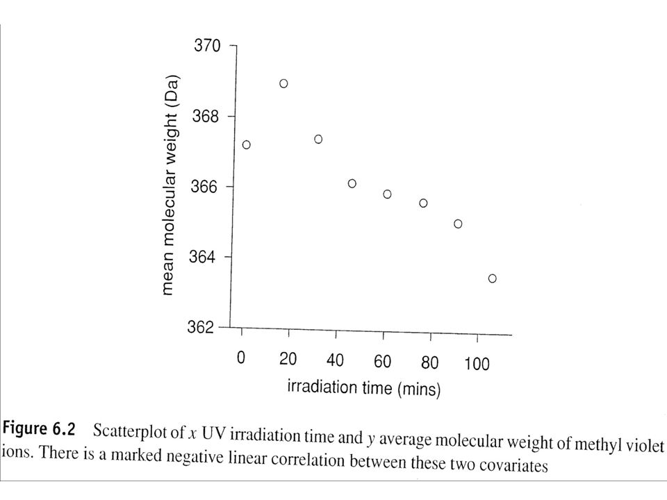
5. Ageing properties of the dye methyl violet (Grim et al., 2002) This example will be used to demonstrate the process involved in the calculation of a linear correlation coefficient Laser desorption mass spectrometry was used to examine the ageing properties of the dye methyl violet, a dye used in inks from the 1950s. Documents written in methyl violet ink were artificially aged with ultra violet radiation. After various times the average molecular weight for the methyl violet compound was measured. The raw data is shown in table 6.1, and plotted in figure 6.2

6. Table 6.1. Average molecular weight of the dye methyl violet and UV irradiation time from an accelerated ageing experiment. Time (min)Weight (Da) 0.0367.20 15.3368.97 30.6367.42 45.3366.19 60.2365.91 75.5365.68 90.6365.12 105.7363.59

8. Correlation coefficient r Visual inspection of Fig. 6.2 suggests that there is a negative linear correlation between time and mean molecular weight. A suitable measure of this linear correlation r is:

9. . Time (min) x – mean x (x – mean x)² Weight (Da) y – mean y (y – mean y)² (x – mean x)(y – mean y) 0.0-52.902798.41367.200.940.883-49.72 15.3-37.611414.51368.972.717.344-101.92 30.6-22.83498.63367.421.161.345-25.90 45.3-7.6157.91366.19-0.070.0050.53 60.27.3353.73365.91-0.350.122-2.57 75.522.61511.21365.68-0.580.336-13.11 90.637.671419.03365.12-1.141.300-42.94 105.752.842792.06363.59-2.677.129-141.08 mean x = 52.89 Σ = 9545.50 mean y = 366.26 Σ = 18.465 Σ = -376.72

10. Substituting these values into the equation for r we have: This means that as the irradiation time increases the average molecular weight of methyl violet ions decreases, and as -0.89 is close to -1, the negative linear relationship is quite strong

11. Significance tests for correlation coefficients A linear correlation coefficient of -0.89 sounds quite high, but is it significantly high? Is it possible that such a coefficient would occur in data drawn randomly from a bivariate normal distribution? Also, what about the effect of sample size? It makes sense that a high coefficient based on lots of x,y pairs is somehow more significant than an equal correlation based on only a few observations. For the null hypothesis that the correlation coefficient is 0, a suitable test statistic is: t = r * √df / √ (1 - r²).

12. Substituting for the methyl violet example t = r * √df / √ (1 - r²). t is the ordinate (horizontal axis) on the t-distribution df is degrees of freedom equal to n – 2 (here = 6 because we have 8 x,y pairs) The linear correlation coefficient was -0.89, so: t = -0.89 * √6 / √ (1 - -0.89²) = -4.78 If we look at the values of the t-distribution table for df = 6 we see that 95% of the area is within ± 2.447. Our value of -4.78 is beyond -2.447, so we can say that the correlation coefficient is significant at 95% confidence.

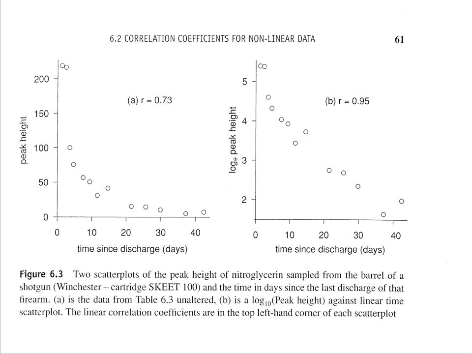
13. Correlation coefficients for non- linear data Andrasko and Ståhling measured three compounds associated with the discharge of firearms, napthalene, TEAC-2 and nitroglycerin over a period of time by solid phase microextraction (SPME) of the gaseous residue from the expended cartridge. They found that the concentrations of these compounds would decrease with time, and that this property would be of use in estimating the time since discharge for this type of cartridges. Table 6.3 is a table of the peak area for nitroglycerine and time elapsed since discharge for a Winchester SKEET 100 cartridge stored at 7°C, shown as scatterplots in Figure 6.3

14. Time since discharge (days) Nitroglycerin (peak height) 1.21218.34 2.42216.16 3.62100.00 4.6975.55 7.4956.52 9.4250.62 11.6031.00 14.6941.44 21.5015.53 25.7014.63 29.8610.41 37.205.16 42.427.26

16. Log-linear relationships A common model for loss in chemistry (e.g. radioactive decay) is called inverse exponential decay, which entails a log-linear relationship between the two variables The right hand scatterplot of Figure 6.3 shows the log to the base e (or natural logarithm) of the nitroglycerine peak height against time. Here we can see that the data looks much more linear. The linear correlation coefficient is -0.95, which is quite high, and suggests that this may be a reasonable transformation of the variables The calculations for the log-linear correlation coefficient are exactly the same kind as in table 6.2, only the log to the base e of the y variable has been used, rather than the untransformed y.

17. The coefficient of determination The coefficient of determination is a direct measure of how much the variance in one of the covariates is attributed to the other. We can imagine that the total variance in the nitroglycerin peak is made up of two parts, that which is attributable to the relationship with x (time), and that which can be seen as random noise. The coefficient of determination describes what proportion of the variance is attributable to relationship with time. The coefficient of determination is simply the square of the correlation coefficient. If r = - 0.95, r² = 0.90. Often the coefficient of determination is described as a percentage, which in the example above would mean that 90% of the variance in nitroglycerin peak area is attributable to time.