1. Vidna kognicija II Danko Nikolić

2. Teme Neurofiziološki kodovi prijenosa i obrade informacija u vidnom sustavu Dva kôda za percepciju svjetline Problem povezivanja dijelova vidne scene u cjelinu (tzv. binding problem) Uloga pažnje u pohranjivanju informacija u radno pamćenje Uloga radnog pamćenja za formiranje dugoročnog vidnog pamćenja Mehanizmi sinestezijskih asocijacija

3. Visual cognition

4. Memory for visual objects:

5. The modal model of memory Sensory memory (iconic memory) Short-term memory (working memory) Long-term memory 200-300 ms Several seconds or while rehearsing Up to life long

6. Objects can have different familiarity... FamiliarNovel

7. … and different complexity. ComplexSimple

8. Long-term memory

9. Short-term memory (Working memory) Luck & Vogel, 1997 Wheeler & Treisman, 2002

10. Detection of visual objects requires attention Feature binding theory Pop-out Lack of pop-out Pop-out Stimulus size Automatic processing Search time Focused attention No pop-out

11. Two different processes: AutomaticAttentive

15. Short presentation X T R P X

16. Short presentation X T R P X

17. Short presentation X T R P X

18. Luck & Vogel, 1997 Conclusion: the capacity of visual WM is about four objects, while every object can consist of multiple features. - WM similar to attention. StudyTest

19. Wheeler & Treisman, 2002 StudyTest Conclusions: - Feature dimensions are independent. - Only four features per feature dimension. - Attention binds features within WM. - Proof: With distractors memory for conjunctions impaired. Performance drops for conjunctions but not for features.

20. G.A. Alvarez and P. Cavanagh The Capacity of Visual Short-Term Memory Is Set Both by Visual Information Load and by Number of Objects, Psychological Science, 2004

22. Henrik Olsson* and Leo Poom Visual memory needs categories, PNAS 2005

23. What about LTM? Hypotheses: –The same attentional mechanisms that bind objects for perceptual purpose also store the binding information into LTM. –WM plays central role in the formation of LTM. –Therefore, formation of LTM for visual objects is limited in the capacity; more complex objects are stored by a serial process.

24. More hypotheses: –The formation of LTM is limited by the capacity of attention to bind features. –The capacity of attention is equivalent to the capacity of WM to store bindings. –Thus, changes in the capacity of attention, change the capacity of WM. WMAttention LTM

25. Stimuli

26. The paradigm

27. Strategy Target Distractor Test array Sample array

28. Two memorization alternatives WM ‘slots’ Chunking Visual object

29. Manipulation of pop-out Why is lack of pop-out needed? –Subjects might chunk with pop-out but not without pop-out. –In this case, formation of LTM is not formed by the same attentional mechanisms that operate during visual search (lack of pop-out). –Alternatively, there is no difference between pop-out and no pop-out in the ability to form LTM.

30. Experiment 1: The capacity of visual WM Short presentation time (1000 ms). Four perceptual conditions. Adaptive change in the array size. –(correct response > increase by 1 element). 150 trials. Starting from small array size of 7 elements. 7 subjects.

31. Array growth in exp. 1 4.1 target locations 1.4 target locations

32. Probability to give a correct response: Pc Number of correctly stored elements: N Total number of elements: S The probability of giving the correct response by guessing: Pg Probability of giving the correct response: Pc = N /S + Pg (1-N /S). Pg = 0.5 Related to model of Pashler (1988) The expected change in array size in a single trial E{ΔS} = E{Increase} + E{Decrease}, which leads to E{ΔS} = 2 Pc – 1. It follows that: E{ΔS} = N /S.

33. Conclusions from exp. 1 WM capacity is narrowly limited. Without distractors WM capacity is not so limited. Thus, the reason is the presence of distractors. This is supported by the further decrease in the capacity without lack of pop-out. The capacity of WM depends on the binding capacity of visual attention: –With pop-out, about four objects. –Without pop-out, fewer objects.

34. Shape II Non pop-out Location Shape If bindings are created in both conditions, there will be no qualitative difference difference between pop-out and no pop-out conditions in the formation of LTM. Pop-out Location Shape

35. Experiment 2: Chunking unlimited presentation time. –dependent variable. 2 sessions, 50 trials each. Fixed array sizes (10, 15, 20 and 25 elements). 2 perceptual conditions (pop-out; no pop-out). 6 subjects.

36. Results exp. 2

37. Encoding times, exp. 2 Sequential (serial) encoding in both conditions. Formation of objects (chunks) is a capacity limited process. Similarly dependent on pop-out as the capacity of WM.

38. WM capacity predicts chunking speed S P = 1345 ms/elem. S NP = 3781 ms/elem.

39. Conclusions exp. 2 The speed of object formation (chunking) depends on the capacity of WM. Thus, the contents of WM are integrated in parallel – one chunking step. The remaining elements are integrated by repeating the chunking steps.

40. Experiment 3: LTM Same as exp. 2 + unexpected LTM test. 10 chunking followed by 10 trials of LTM test. 2 conditions: Small and larger array (WM vs. chunk). 8 subjects (4 in each condition).

41. Results exp. 3

42. Conclusions When storing bindings, the capacity of WM depends on the binding capacity of visual attention (magic number 4). Subjects exceed the capacity of WM by storing visual objects (chunks) in LTM. No qualitative difference between pop-out and non pop-out conditions in the formation of LTM (always a sequential process; no change in strategy). The only difference is in the speed of the sequential process. The differences in the speed can be explained by the capacity of visual WM for the same stimuli. The working component of WM is visual attention. WM and attention jointly store the binding information into LTM, enabling thus storage of visual objects.

44. Figure 2. The procedure used in Experiment 1. Participants detected the target items and memorized the shapes surrounding them. The presentation time that was needed to achieve high WM performance was determined by the participants themselves. After an interval of 8 s participants had to judge whether the test shape matched one of the target shapes. ITI: Inter-trial interval.

45. Figure 3. Results from Experiment 1. A. Mean response accuracy at test as a function of WM load and attentional demand. B. Mean presentation times as a function of WM load and attentional demand (PO: pop-out; NPO: non pop-out). Vertical bars: the standard error of the mean.

46. Figure 4. The procedure used in Experiment 2. Participants detected and counted the target items. After pressing the response button a question mark appeared prompting the participants to enter the number of the counted targets. ITI: Inter- trial interval.

47. Figure 5. Results from Experiment 2. A. Mean response accuracy at test as a function of WM load and attentional demand. B. Mean counting times as a function of WM load and attentional demand (PO: pop-out; NPO: non pop-out). Vertical bars: the standard error of the mean.

48. Experiment 3: Information about the upcoming number of targets.

49. Figure 6. Results from Experiment 3 compared to the results from Experiment 1. A. Mean response accuracy at test as a function of WM load and attentional demand. B. Mean presentation times as a function of WM load and attentional demand (PO: pop-out; NPO: non pop-out). C. Differences in the presentation times between pop-out and non pop-out conditions across WM load conditions. Vertical bars: the standard error of the mean.

50. Figure 6. C. Differences in the presentation times between pop-out and non pop-out conditions across WM load conditions. Vertical bars: the standard error of the mean.

51. Figure 7. A. Empirically obtained offset in the presentation times produced by lack of pop-out in Experiment 3 and theoretically predicted offset based on search times from Experiment 2, computed for five different memory loads. B, Offset in the presentation times produced by lack of pop-out that is not explained by the visual search and that is expressed as a function of the number of target items. Dashed line: linear fit (see text).

52. Figure 8. The procedure used in Experiment 4. Participants detected the target items and memorized their locations only. After an interval of 8 s participants judged whether the location of the missing item in the test array matched one of the target locations. ITI: Inter-trial interval.

53. Figure 9. Results from Experiment 4. A. Mean response accuracy at test as a function of WM load and attentional demand. B. Mean presentation times as a function of WM load and attentional demand (PO: pop- out; NPO: non pop-out). Vertical bars: the standard error of the mean.

54. Experiment 5: same as experiment 4 but with knowing the upcoming number of targets (as in experiment 3).

55. Figure 10. Results from Experiment 5 compared to the results from Experiment 3. A. Mean presentation times as a function of WM load and attentional demand (PO: pop-out; NPO: non pop-out). B. Differences in the presentation times between pop-out and non pop-out conditions across WM load conditions. Vertical bars: the standard error of the mean. C. Offset in the presentation times produced by lack of pop-out that is not explained by the visual search and that is expressed as a function of the number of target items. Dashed lines: linear fit.

56. Figure 10. C. Offset in the presentation times produced by lack of pop-out that is not explained by the visual search and that is expressed as a function of the number of target items. Dashed lines: linear fit.

57. Conclusions WM and attention interfere and perhaps use the same resources. Memory for locations prevents interference.

58. Funkcionalna magnetska rezonanca

61. BOLD signal

62. Attentional Demand Influences Strategies for Encoding into Visual Working Memory Jutta S. Mayer1, Robert A. Bittner1, David E. J. Linden1, 2 and Danko Nikolić3, 4 (under review)

65. Information maintenance

69. Kraj kognitivnog dijela

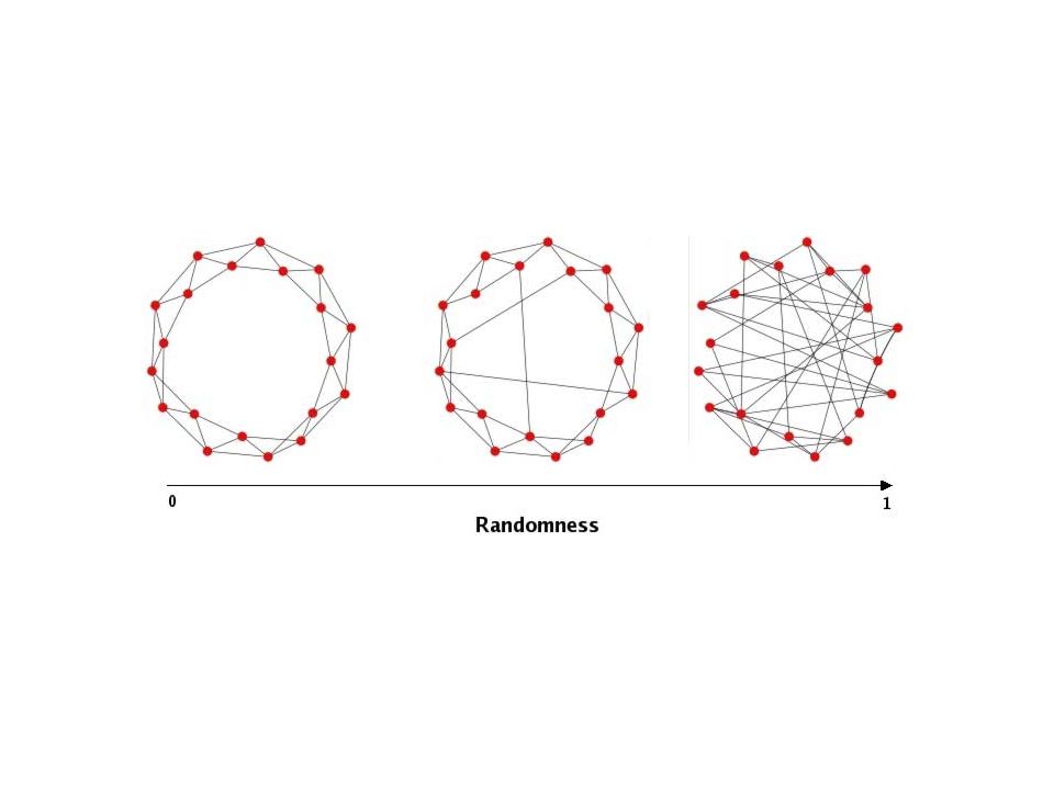
70. Mreže maloga svijeta (small-world networks)

71. Small world networks Stanley Milgram (1967) Watts and Strogatz (1998)

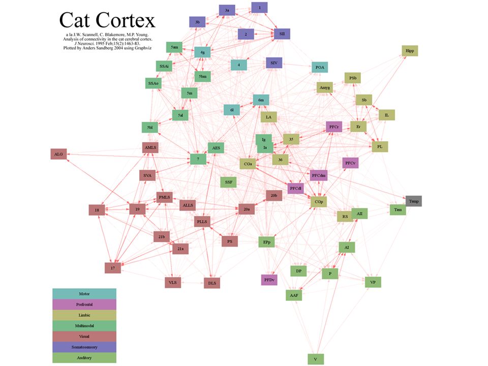
75. A small world of neuronal synchrony

76. A small world network A small-world network partially shares properties with random networks, which have short average path lengths (i.e., any pair of nodes is likely to be connected through a small number of other nodes) … and partially also with regular networks, which are organized into clusters (i.e. a high level of local interconnectivity). A small-world property: the same average path lengths as random networks, λ ≈ 1, but empirical network should have a larger clustering coefficient than a random network, γ > 1.

78. Applying Ising model to estimate neuronal interactions

79. Bottom-up Common input Input is not shared

80. Lateral interactions Tangential connections

81. Top-down Lower visual areaHigher visual area Feedback connections

82. Applying Ising model to estimate neuronal interactions

83. A small world of neuronal synchrony Clustering coefficient