Download presentation
Presentation is loading. Please wait.

1
Adventures in Parameter Estimation Jason Dick University of California, Davis

2
Motivation Goal: to gain information about basic physics through parameter estimation. Two major areas that have significant open questions today are dark energy and inflation. Upcoming experiments have the capability to provide significant information about the physics of these phenomena.

3
Inflation Best experimental test currently available for inflation is the Cosmic Microwave Background. Recent tentative detection of a departure from scale invariance in the three-year WMAP data release begs for further investigation. –Interesting because we expect some small departure from scale invariance for most inflationary models. One way of measuring this better is to measure higher multipoles more accurately, as we will be doing with the SPT project.

4
Dark Energy Is dark energy a cosmological constant? Theory gives little insight as to how dark energy varies. Theory-independent analysis. –Want to look at those types of variation best- constrained by the data. Our solution: use eigenmodes.

5
What we found Our method appears to be an optimal method for detecting dark energy variation. But the eigenmodes we found cannot be physical. –Variation is too fast at the one-sigma error level to be explained by dark energy. So for now, just a systematic error test. When future data place better constraints on the eigenmodes, there will be a possibility of detecting real variation.

6
Data Supernova data: Riess et. al. (astro- ph/0402512) and Astier et. al. (astro- ph/0510447) WMAP constraints: Obtained from chain available at the LAMBDA archive (http://lambda.gsfc.nasa.gov) BAO constraints: Eisenstein et. al. (astro- ph/0501171)
 WMAP constraints: Obtained from chain available at the LAMBDA archive ( BAO constraints: Eisenstein et. al. (astro- ph/ ).")
7
Parameterization Define: ρ x (z) = ρ c (0)a i e i (z). Choose basis: e 0 is constant, others vary Constant basis vector One varying vector Another varying vector

8
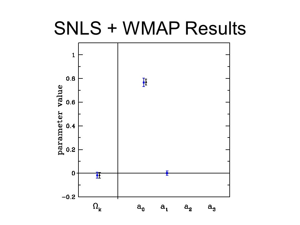
Diagonalization To describe our cosmology, we now have the parameters: ω m, Ω k, a 0, a 1 -a n, and the supernova parameters: M, α, β. Take Gaussian approximation to marginalize over all but a 1 -a n. Diagonalize to get eigenvectors (a new basis):
:.")
9
Some example eigenmodes First varying mode Second varying mode Third varying mode

10
MCMC Analysis Don’t want to be limited by the Gaussian approximation. Using MCMC, estimate values and errors of best-measured modes only. The errors in each varying mode should be uncorrelated with all other varying modes.

11
SNLS + WMAP Results

15
When Gaussians Go Bad Adding more modes: degeneracies appear. Here it happens when the MCMC chain includes the 7 th dark energy parameter. Four leftmost of each group of parameters are very poorly- constrained: some are off the graph! SNLS + BAO + WMAP

16
But is the variation too fast? 1-σ Variation of Eigenmodes

17
Why is this method useful? Estimation of energy density directly, instead of through integration of w(z), should result in tighter constraints on the density. Any real variation of dark energy should show up in the first eigenmode, as higher eigenmodes vary more quickly and are less likely to describe real physics. Use of eigenmode analysis should ensure that if the data can detect variation in dark energy, it should be detected by this method. –This bears investigation, however.
, should result in tighter constraints on the density. Any real variation of dark energy should show up in the first eigenmode, as higher eigenmodes vary more quickly and are less likely to describe real physics. Use of eigenmode analysis should ensure that if the data can detect variation in dark energy, it should be detected by this method. –This bears investigation, however..")
18
Possible issues The eigenmodes in dark energy density do not have an obvious connection with physics: this test only addresses the question as to whether or not dark energy varies, but the connection to specific dark energy models is not clear at this point. Have not tested method against many simulated data sets with different sorts of varying dark energy. –Main problem: how to allow dark energy to vary in many different ways without biasing models?

19
Results of Dark Energy Analysis Good method for detecting deviation from constant without being tied to a particular theory. MCMC analysis is self-checking. No detected variation: systematic error test passed. We expect this technique to be excellent at discovering whether or not we have a cosmological constant for future data.

20
Moving on to Inflation Any questions before we continue?

21
South Pole Telescope: Measuring the CMB at high resolution Instrument: –960 bolometer array –4000 deg 2 survey area –Arcminute resolution Benefits for CMB science: –Large sky coverage will allow highly accurate calibration with WMAP (and later Planck) results. –High resolution allows measurement of primary CMB to high multipoles (up to about l =3000-4000).
..")
22
What does this mean for constraining Inflation? Lloyd Knox, 2006

23
Obtaining Cosmological Parameters Method is straightforward: libraries such as CMBEASY and CMBFAST are available and easy to use. But we need to develop a likelihood estimator for SPT data. Requires estimation of power spectrum and errors on the power spectrum.

24
Estimating the Power Spectrum Use MASTER-like algorithm, as described in Hivon et. al. (astro-ph/0105302). Algorithm parameterizes the power spectrum as follows: Pseudo C l method first estimates the power spectrum of the map through a direct spherical harmonic transform, then compares it against a theory power spectrum that has been modified in the above way. –Method pioneered by Gorski in astro-ph/9403066
. Algorithm parameterizes the power spectrum as follows: Pseudo C l method first estimates the power spectrum of the map through a direct spherical harmonic transform, then compares it against a theory power spectrum that has been modified in the above way. –Method pioneered by Gorski in astro-ph/")
25
Calculating M ll’ Calculation assumes statistical isotropy –Can we relax this? –May not need to.

26
Testing M ll ’ on 1000deg 2 map

27
Estimating F l Want to use Monte Carlo techniques to find F l. –Will be computationally difficult to simulate for every l value. –Define F l at discrete l values. –Interpolate in between using cubic interpolation.

28
Still to come Estimating the beam profile contribution B l –Described in Wu et. al. 2001 (astro-ph/0007212). Estimating the noise contribution N l –Described in Hivon et. al. 2002 (astro-ph/0105302).
. Estimating the noise contribution N l –Described in Hivon et. al (astro-ph/ )..")
29
Next step: Simulating the detectors Computationally intensive. –960 detectors! –Use small maps to start Atmosphere model –Modeled as a smooth gradient in temperature that slowly moves across the field with time. –First approximation: remove with high-pass filter. –May implement more careful sky removal later. Detector noise –Modeled as white + 1/f Point sources –Can mask these out, so can simulate their effect by arbitrarily masking a few small regions on the map. Diffuse galactic sources –Purposely measuring in area with low emission in our frequency bands.

30
WMAP dust map (W-band) Courtesy: WMAP Science Team Linear scale, -0.5 – 2.3 mK
 Courtesy: WMAP Science Team Linear scale, -0.5 – 2.3 mK")
31
Conclusions SPT will allow for excellent measurement of deviation from scale invariance. Highly complementary with current and future CMB experiments, such as WMAP, ACT, and Planck. Going online this summer!

Similar presentations


 I Workshop “Challenges.>")


, J. Richard Gott.>")

 with George Efstathiou (Cambridge University) Efstathiou &>")


 Currently Astrophysics Group (Cavendish Lab., Cambridge) Wiaux, Vielva, Martínez-González.>")

 CCAPP, 23 June 2010.>")


