1. Artificial Intelligence University Politehnica of Bucharest 2007-2008 Adina Magda Florea http://turing.cs.pub.ro/ai_07

2. Lecture No. 2 Problem solving strategies Representing problem solution Basic search strategies Informed search strategies

3. 1. Representing problem solution Symbolic structure Computational instruments Planning method / approach

4. 1.1. State space representation state, state space, initial state, final state(s), operators (S i, O, S f ) Problem solution

5. 8-puzzle

6. 1.2 AND/OR graph representation Problem decomposition into sub-problems (P i, O, P e ) AND/OR graph Solved node Unsolvable node Problem solution

7. AND/OR graph OR AND

8. Towers of Hanoi

9. 1.3 Equivalence of representations State space Problem decomposition

10. 2. Basic search strategies Criteria Completeness Optimality Complexity Possibility to backtrack Informedness Conventions: unknown node, evaluated node, expanded node, OPEN, CLOSED

11. Computational costs of search

12. 2.1. Uninformed search in state space Algorithm BREADTH:Breadth first search in state space 1.Init lists OPEN  {S i }, CLOSED  {} 2.if OPEN = {} then return FAIL 3.Remove first node S from OPEN and insert it in CLOSED 4.Expand node S 4.1.Generate all direct successors S j of node S 4.2.for each successor S j of S do 4.2.1.Make link S j  S 4.2.2.if S j is final state then i.Solution is (S j, S,.., S i ) ii.return SUCCESS 4.2.3.Insert S j in OPEN, at the end 5.repeat from 2 end.

13. Features of breadth first search Previous algorithm for tree space not graph For graphs - Insert step 3’ 3’.if S  OPEN  CLOSED then repeat from 2 Depth first search in state space Depth of a node Ad(S i ) = 0, where S i is the initial state, Ad(S) = Ad(S p )+1, where S p is the predecessor node of S.

14. Algorithm DEPTH(AdMax): Depth first search in state space 1.Init lists OPEN  {S i }, CLOSED  {} 2.if OPEN = {} then return FAIL 3. Remove first node S from OPEN and insert it into CLOSED 3’. if Ad(S) = AdMax then repeat from 2 4.Expand node S 4.1.Generate all successors S j of node S 4.2.for each succesor S j of S do 4.2.1.Set link S j  S 4.2.2.if S j is final state then i.Solution is (S j,.., S i ) ii.return SUCCESS 4.2.3.Insert S j in OPEN, at the beginning 5.repeat from 2 end.

15. Features of depth first search Iterative deepening for AdMax=1, Val do DEPTH(AdMax) Features of iterative deepening Bidirectional search Which strategy to choose ?

16. 2.2. Uninformed search in AND/OR graphs Depth of a node Ad(S i ) = 0, where, S i is the node of the initial problem Ad(S) = Ad(S p ) + 1 if S p is node OR predecesor of node S, Ad(S) = Ad(S p ) if S p is node AND predecesor of node S.

17. Algorithm BREADTH-ANDOR:Breadth first search in AND/OR trees 1.Init lists OPEN  {S i }, CLOSED  {} 2.Remove first node S from OPEN and insert it into CLOSED 3.Expand node S 3.1.Generate all direct successors S j of node S 3.2.for each successor S j of S do 3.2.1.Make link S j  S 3.2.2.if S j is a set of at least 2 sub-problems then/* is an AND node*/ i.Generate all successors sub-problems S k j of S j ii.Set link S k j  S j iii.Insert nodes S k j in OPEN, at the end 3.2.3.else Insert S j in OPEN, at the end

18. 4.if no successor of S was generated in previous step (3) then 4.1. if S is terminal node labeled with a non-elementary problem then 4.1.1.Label S unsolvable 4.1.2.Label with unsolvable all nodes predecessor of S which become unsolvable because of S 4.1.3.if node AND is unsolvable then return FAIL/* no solution */ 4.1.4.Remove from OPEN all nodes which have unsolvable predecessors 4.2. else/* S is terminal node labeled with a non-solvable problem */ 4.2.1.Label S solved 4.2.2.Label with solved all nodes predecessor of S which become unsolvable because of S 4.2.3.if node AND is solved then i. Build solution tree following the links ii. return SUCCESS/* Solution found */ 4.2.4.Remove from OPEN all solved nodes and all nodes which have solved predecessors 5.repeat from 2 end.

19. 2.3. Complexity of search strategies B – branching factor of the search space 8-puzzle Number of moves: 2 m for corners = 8 3 m for laterals = 12 4m for center  24 moves B = no. moves / no. pozitions of free square = 2.67 Number of moves : 1 m for corners = 4 2 m for laterals = 8 3m for center  15 moves  B = 1.67

20. Complexity of search strategies B - branching factor Root – B nodes, B 2 on level 2, etc. Number of states possible to be generated on a search level d is B d T – total number of states generated during a search, d – depth of solution node T = B + B 2 + … + B d = O(B d )

21. Number of generated nodes Breadth first search B + B 2 + … + B d + (B d+1 -B) = O(B d+1 ) B – branching factor, d – depth of solution Depth first search B - branching factor, m – maximum depth B*m+1 Iterative deepening search d*B+(d-1)*B 2 + … + (1)*B d = O(B d )

22. Complexity of search strategies CriterionLevelDepthLimited depth Iterative deepening Bidirectio nal TimeBdBd BmBm BlBl BdBd B d/2 SpaceBdBd B*mB*lBdBd B d/2 Optimality ? YesNo Yes Completen ess YesNo Yes if l  d Yes B – branching factor, d – solution depth, m – maximum depth of the tree, l –limit of search (AdMax)

23. 3. Informed search strategies Use heuristic knowledge to incraese efficiency of search: Select which node to expand nex during search While expanding a node decide which successors to generate and which to ignore Remove from the search space some nodes that have previously been generated – prune the search space

24. 3.1 Best-first search Evaluate the information that can be obtained by expanding a node and ist importance in guiding the search The quality of a node is estimated by the heuristic search function w(n) for node n hill climbing strategy best-first strategy

25. Algorithm BFS:Best-first in state space 1.Init lists OPEN  {S i }, CLOSED  {} 2.Compute w(S i ) and associate this value to S i 3.if OPEN = {} then return FAIL 4. Remove node S with minimum w(S) from OPEN and insert it in CLOSED 5.if S is final state then i.Solution is (S,.., S i ) ii.return SUCCESS 6.Expand node S 6.1. Generate all successors S j of node S 6.2. for each succesor S j of S do 6.2.1Compute w(S j ) and associate it to S j 6.2.2.Set link S j  S

26. 6.2.3.if S j  OPEN  CLOSED then insert S j in OPEN with associated w(S j ) 6.2.5.else i. Be S’ j the copy of S j from OPEN or CLOSED ii. if w(S j ) < w(S’ j ) then - Remove link S’ j  S p, with S p pred. of S’ j - Set link S’ j  S, and update cost of S’ j to w(S j ) - if S’ j is in CLOSED - then remove S’ j from CLOSED and insert S’ j in OPEN iii. else ignore node S j 7.repeat from 3 end.

27. Cases Best-first strategy is a generalization of uninformed search strategies - Breadth first search w(S) = Ad(S) - Depth first search w(S) = -Ad(S) Uniform cost strategy Minimize the search effort – heuristic search w(S) = heuristic function

28. 3.2 Optimal solutions: A*Algorithm w(S) becomes f(S) with 2 components: g(S), estimates the real cost g*(S) of the search path from S i to S, h(S), estimates the real cost h*(S) of the search path from S to S f. f(S) = g(S) + h(S) f*(S) = g*(S) + h*(S)

29. Components of A*

30. Computing f(S) Computation of g(S) Computation of h(S) Must be admissible A heuristic function is called admissible if for any state S, h(S)  h*(S). This definition gives the admissibility condition of function h and is used to define the property of admissibility of an algorithm A*.

31. A* admissibility Consider an algorithm A* which uses g and h compenents of f if (1)h satisfies the admissibility condition (2) for any 2 states S, S', where c > 0 is a constant and the cost is finite then A* algorithm is admissible, i.e., is guaranteed to find the path of minimal cost to solution. Completeness

32. Implementation of A* Modify the algorithm correspnding to the "best-first" strategy in state space as such: … 2.Compute w(S i )=g(S i ) + h(S i ) and associate this value to S i 3.if OPEN = {} then return FAIL - unmodified 4. Remove node S with w(S) minimum from OPEN and insert it into CLOSED - unmodified ….. 6.2.5.else i. Be S’ j the copy of S j from OPEN or CLOSED ii. if g(S j ) < g(S’ j ) then …

33. The heuristic of A* Consider 2 algorithms A*, A1 and A2, with evaluation functions h 1 and h 2 admissibile, g 1 =g 2 It is said that A2 is more informed than A1 if for any state S with S  S f We say that h2 dominates h1 monotony

34. How we compute f 8-puzzle Traveling salesman h2(S) = the cost of the minimum spanning tree of unvisited cities until S

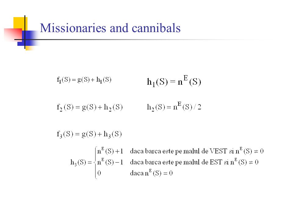
35. Missionaries and cannibals

37. Relaxing the admissibility condition of A* An heuristic function h is called  -admissible if with  > 0 An A* algorithm which uses an evaluation function f with a component h  -admissible will find a solution which has a cost greater than the cost of the optimal solution with at most . such an algorithm - an  -admissible algorithm and the solutions is called  -optimal solution.

38. Relaxing the admisibility condition of A* 8-puzzle

39. Recursive Best First Best first with linear space Recursive implementation Remembers the value f of the best alternate path which starts from any precedent node of the current node Finds the minimum cost solution if h is admissible but has a space complexity of O(B*d)

40. S1 S3 S8 S5 S2 S6 S7 S4 S9 S10S11 447 449 inf 393 646 415 526 413 526 417 553 415 S1 S3 S8 S5 S2 S6 S7 S4 S12S13 447 449 inf 393 646 415 526 417 450 591 417

41. S1 S3 S8 S5 S2 S6 S7 S4 S9 S10S11 447 449 inf 393 646 450 526 417 526 417 553 447 S14S15 615 418 S16 607 447 BestFR(S) Recursive Best First strategy /* returns the solution or FAIL */ BFR(Si, inf)

42. Algorithm BFR(S, f_lim): Recursive Best First strategy /* Returns a solution or FAIL and a new limit f_limit */ 1. if S final state then return S, f_lim 2. Generate all successors S j of S 3. if there are no successors then return FAIL, inf 4. for each successor Sj do f(S j )  max(g(S j ) + h(S j ), f(S)) 5. Best  S j min, node with minimal value f(S j ) among successors 6. if f(Best) > f_lim then return FAIL, f(Best) 7. Alternat  f(S j min2 ), the 2 nd smallest value f(S j ) 8. Rez, f(Best)  BFR(Best, min(f_lim, Alternat) 9. if Rez  FAIL then return Rez, f(Best) 10. repeat from step 5 end.