2. NEW FRONTIERS FOR ARCH MODELS Prepared for Conference on Volatility Modeling and Forecasting Perth, Australia, September 2001 Robert Engle UCSD and NYU

3. The First ARCH Model  Rolling Volatility or “Historical” Volatility Estimator – Weights are equal for j<N – Weights are zero for j>N – What is N?

4. 1982 ARCH Paper  Weights can be estimated  ARCH(p)

5. WHAT ABOUT HETEROSKEDASTICITY?

6. EXPONENTIAL SMOOTHER  Another Simple Model – Weights are declining – No finite cutoff – What is lambda? (Riskmetrics=.06)

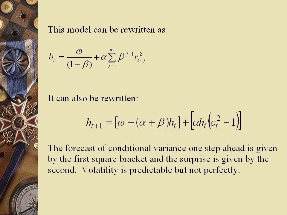
7. The GARCH Model   The variance of r t is a weighted average of three components – a constant or unconditional variance – yesterday’s forecast – yesterday’s news

10. FORECASTING WITH GARCH  GARCH(1,1) can be written as ARMA(1,1)  The autoregressive coefficient is  The moving average coefficient is

11. GARCH(1,1) Forecasts

12. Monotonic Term Structure of Volatility

13. FORECASTING AVERAGE VOLATILITY  Annualized Vol=square root of 252 times the average daily standard deviation  Assume that returns are uncorrelated.

14. TWO YEARS TERM STRUCTURE OF PORT

16. Variance Targeting  Rewriting the GARCH model  where is easily seen to be the unconditional or long run variance  this parameter can be constrained to be equal to some number such as the sample variance. MLE only estimates the dynamics

17. The Component Model  Engle and Lee(1999)  q is long run component and (h-q) is transitory  volatility mean reverts to a slowly moving long run component

18. MORE GARCH MODELS  CONSIDER ONLY SYMMETRIC GARCH MODELS  ESTIMATE ALL MODELS WITH A DECADE OF SP500 ENDING AUG 2 2001  GARCH(1,1), EGARCH(1,1), COMPONENT GARCH(1,1) ARE FAMILIAR

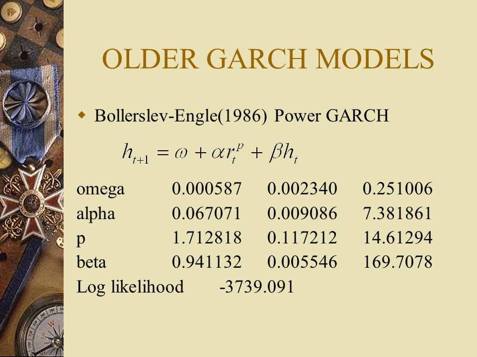
20. OLDER GARCH MODELS  Bollerslev-Engle(1986) Power GARCH omega0.0005870.0023400.251006 alpha0.0670710.0090867.381861 p 1.7128180.11721214.61294 beta0.9411320.005546169.7078 Log likelihood-3739.091

21. PARCH  Ding Granger Engle(1993) omega0.0066800.0016534.041563 alpha 0.0649300.00560811.57887 gamma0.6656360.0828148.037719 beta 0.9416250.005211180.704 Log likelihood-3738.040

22. TAYLOR-SCHWERT  Standard deviation model omega0.0076780.0016674.605529 alpha0.0652320.00521212.51587 beta 0.9425170.005104184.6524 Log likelihood-3739.032

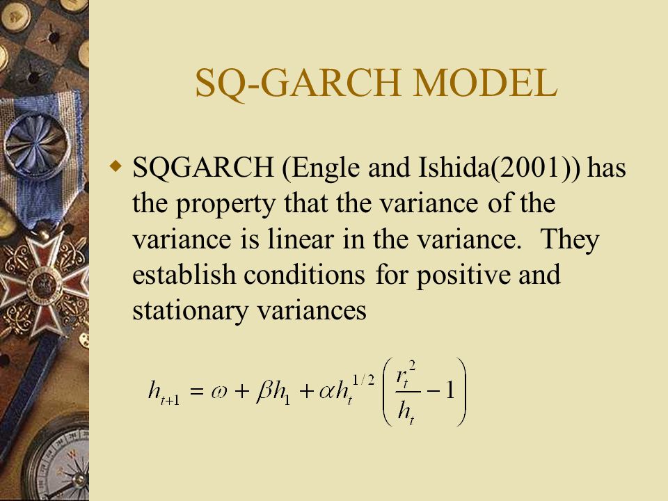
24. SQ-GARCH MODEL  SQGARCH (Engle and Ishida(2001)) has the property that the variance of the variance is linear in the variance. They establish conditions for positive and stationary variances

25. SQGARCH LogL: SQGARCH Method: Maximum Likelihood (Marquardt) Date: 08/03/01 Time: 19:47 Sample: 2 2928 Included observations: 2927 Evaluation order: By observation Convergence achieved after 12 iterations Coefficient Std. Errorz-StatisticProb. C(1)0.0088740.0015965.5602360.0000 C(2)0.0418780.00368511.363830.0000 C(3)0.9900800.001990497.58500.0000 Log likelihood-3747.891 Akaike info criterion2.562960 Avg. log likelihood-1.280455 Schwarz criterion2.569090 Number of Coefs.3 Hannan-Quinn criter.2.565168

26. CEV-GARCH MODEL  The elasticity of conditional variance with respect to conditional variance is a parameter to be estimated.  Slight adjustment is needed to ensure positive variance forecasts.

27. NON LINEAR GARCH  THE MODEL IS IGARCH WITHOUT INTERCEPT. HOWEVER, FOR SMALL VARIANCES, IT IS NONLINEAR AND CANNOT IMPLODE  FOR

28. NLGARCH LogL: NLGARCH Method: Maximum Likelihood (Marquardt) Date: 08/18/01 Time: 11:27 Initial Values: C(2)=0.05464, C(4)=0.00035, C(1)=2.34004 Convergence achieved after 32 iterations CoefficientStd. Errorz-StatisticProb. alpha0.0541960.00474911.411580.0000 gamma0.0012080.0019350.6242990.5324 delta3.1940724.4712260.7143620.4750 Log likelihood-3741.520 Akaike info criterion2.558606 Avg. log likelihood-1.278278 Schwarz criterion2.564737 Number of Coefs.3 Hannan-Quinn criter.2.560814

30. Asymmetric Models - The Leverage Effect  Engle and Ng(1993) following Nelson(1989)  News Impact Curve relates today’s returns to tomorrows volatility  Define d as a dummy variable which is 1 for down days

31. NEWS IMPACT CURVE

32. Other Asymmetric Models

33. PARTIALLY NON-PARAMETRIC ENGLE AND NG(1993)

34. EXOGENOUS VARIABLES IN A GARCH MODEL  Include predetermined variables into the variance equation  Easy to estimate and forecast one step  Multi-step forecasting is difficult  Timing may not be right

35. EXAMPLES  Non-linear effects  Deterministic Effects  News from other markets – Heat waves vs. Meteor Showers – Other assets – Implied Volatilities – Index volatility  MacroVariables or Events

36. STOCHASTIC VOLATILITY MODELS  Easy to simulate models  Easy to calculate realized volatility  Difficult to summarize past information set  How to define innovation

37. SV MODELS  Taylor(1982)  beta=.997  kappa=.055  Mu=0

38. Long Memory SV  Breidt et al, Hurvich and Deo  d=.47  kappa=.6

39. Breaking Volatility  Randomly arriving breaks in volatility  mu=-0.5  kappa=1  p=.99