1. Introduction to Linear Algebra Mark Goldman Emily Mackevicius

2. Outline 1. Matrix arithmetic 2. Matrix properties 3. Eigenvectors & eigenvalues -BREAK- 4. Examples (on blackboard) 5. Recap, additional matrix properties, SVD

3. Part 1: Matrix Arithmetic (w/applications to neural networks)

4. Matrix addition

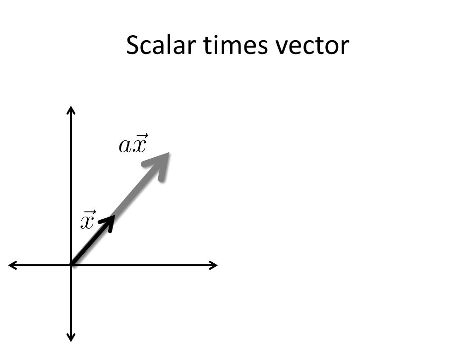
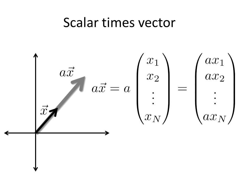
5. Scalar times vector

8. Product of 2 Vectors Element-by-element Inner product Outer product Three ways to multiply

9. Element-by-element product (Hadamard product) Element-wise multiplication (.* in MATLAB)

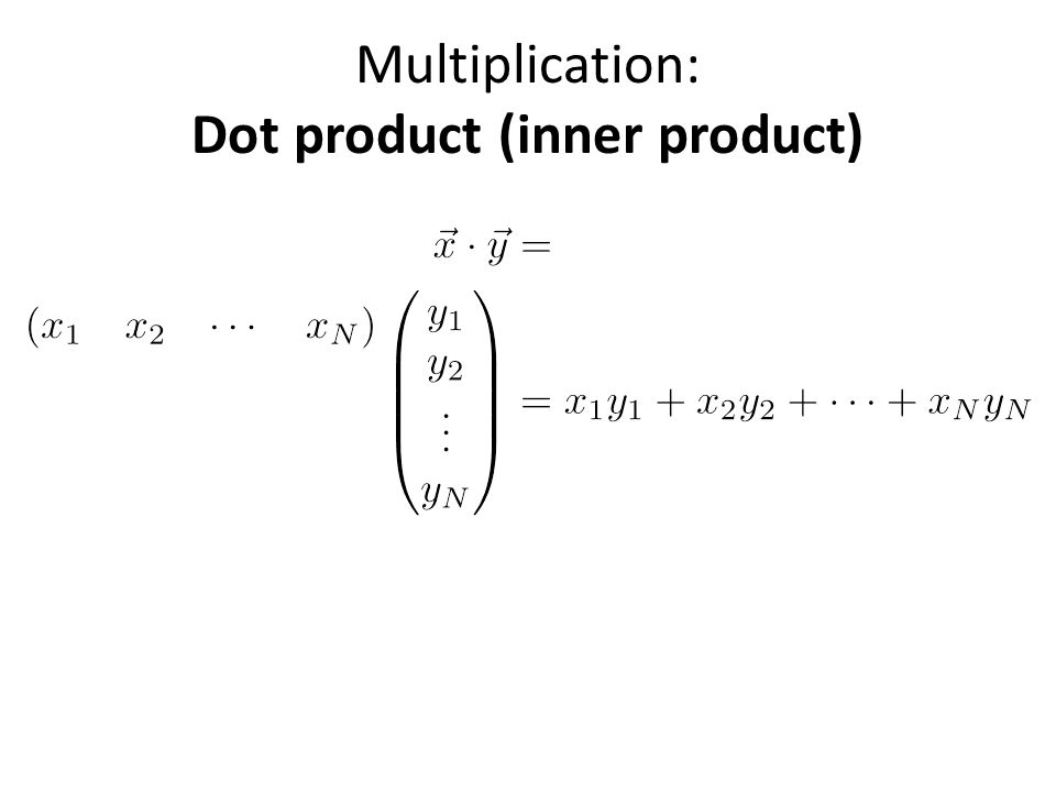
10. Dot product (inner product)

11. Multiplication: Dot product (inner product)

14. 1 X NN X 1 1 X 1 MATLAB: ‘inner matrix dimensions must agree’ Outer dimensions give size of resulting matrix

15. Dot product geometric intuition: “Overlap” of 2 vectors

16. Example: linear feed-forward network Input neurons’ Firing rates r1r1 r2r2 rnrn riri

17. Example: linear feed-forward network Input neurons’ Firing rates Synaptic weights r1r1 r2r2 rnrn riri

18. Example: linear feed-forward network Input neurons’ Firing rates Output neuron’s firing rate Synaptic weights r1r1 r2r2 rnrn riri

19. Example: linear feed-forward network Insight: for a given input (L2) magnitude, the response is maximized when the input is parallel to the weight vector Receptive fields also can be thought of this way Input neurons’ Firing rates Output neuron’s firing rate Synaptic weights r1r1 r2r2 rnrn riri

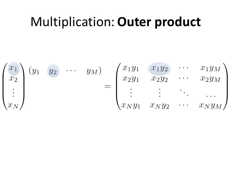
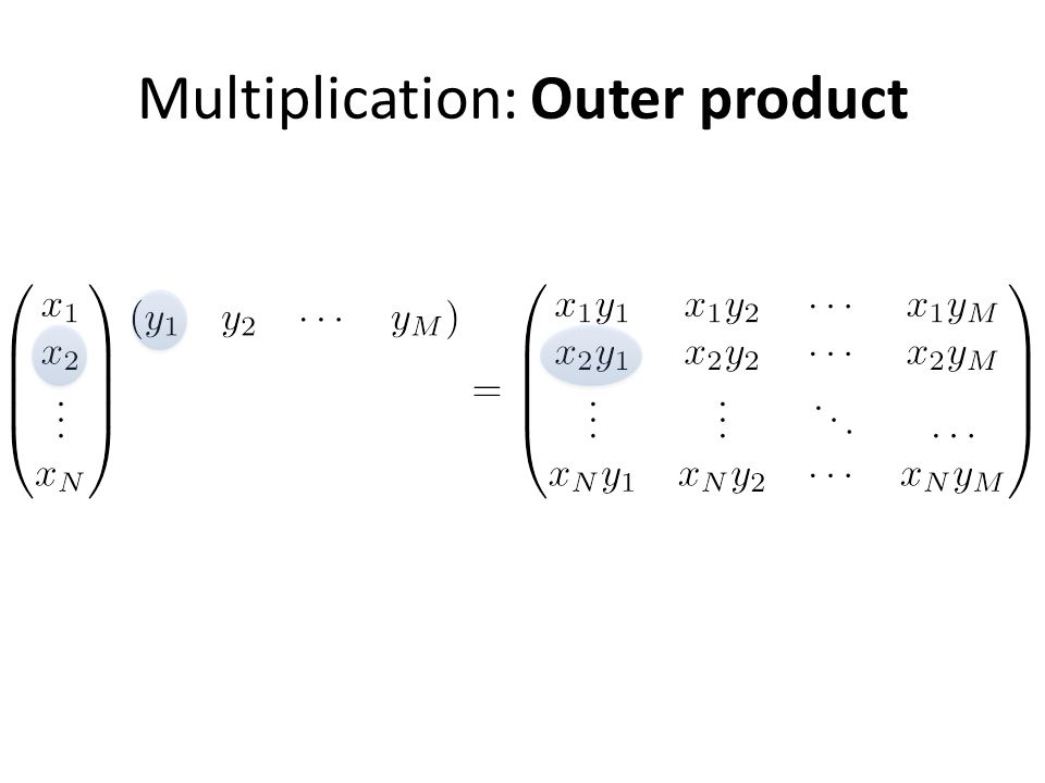
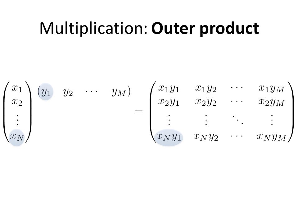
20. Multiplication: Outer product N X 11 X MN X M

21. Multiplication: Outer product

27. Note: each column or each row is a multiple of the others

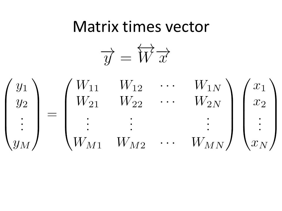
28. Matrix times vector

30. M X 1M X NN X 1

31. Matrix times vector: inner product interpretation Rule: the i th element of y is the dot product of the i th row of W with x

32. Matrix times vector: inner product interpretation Rule: the i th element of y is the dot product of the i th row of W with x

33. Matrix times vector: inner product interpretation Rule: the i th element of y is the dot product of the i th row of W with x

34. Matrix times vector: inner product interpretation Rule: the i th element of y is the dot product of the i th row of W with x

35. Matrix times vector: inner product interpretation Rule: the i th element of y is the dot product of the i th row of W with x

36. Matrix times vector: outer product interpretation The product is a weighted sum of the columns of W, weighted by the entries of x

37. Matrix times vector: outer product interpretation The product is a weighted sum of the columns of W, weighted by the entries of x

38. Matrix times vector: outer product interpretation The product is a weighted sum of the columns of W, weighted by the entries of x

39. Matrix times vector: outer product interpretation The product is a weighted sum of the columns of W, weighted by the entries of x

40. Example of the outer product method

41. (3,1) (0,2)

42. Example of the outer product method (3,1) (0,4)

43. Example of the outer product method (3,5) Note: different combinations of the columns of M can give you any vector in the plane (we say the columns of M “span” the plane)

44. Rank of a Matrix Are there special matrices whose columns don’t span the full plane?

45. Rank of a Matrix Are there special matrices whose columns don’t span the full plane? (1,2) (-2, -4) You can only get vectors along the (1,2) direction (i.e. outputs live in 1 dimension, so we call the matrix rank 1)

46. Example: 2-layer linear network W ij is the connection strength (weight) onto neuron y i from neuron x j.

47. Example: 2-layer linear network: inner product point of view What is the response of cell y i of the second layer? The response is the dot product of the i th row of W with the vector x

48. Example: 2-layer linear network: outer product point of view How does cell x j contribute to the pattern of firing of layer 2? Contribution of x j to network output 1 st column of W

49. Product of 2 Matrices MATLAB: ‘inner matrix dimensions must agree’ Note: Matrix multiplication doesn’t (generally) commute, AB  BA N X PP X MN X M

50. Matrix times Matrix: by inner products C ij is the inner product of the i th row with the j th column

51. Matrix times Matrix: by inner products C ij is the inner product of the i th row with the j th column

52. Matrix times Matrix: by inner products C ij is the inner product of the i th row with the j th column

53. Matrix times Matrix: by inner products C ij is the inner product of the i th row of A with the j th column of B

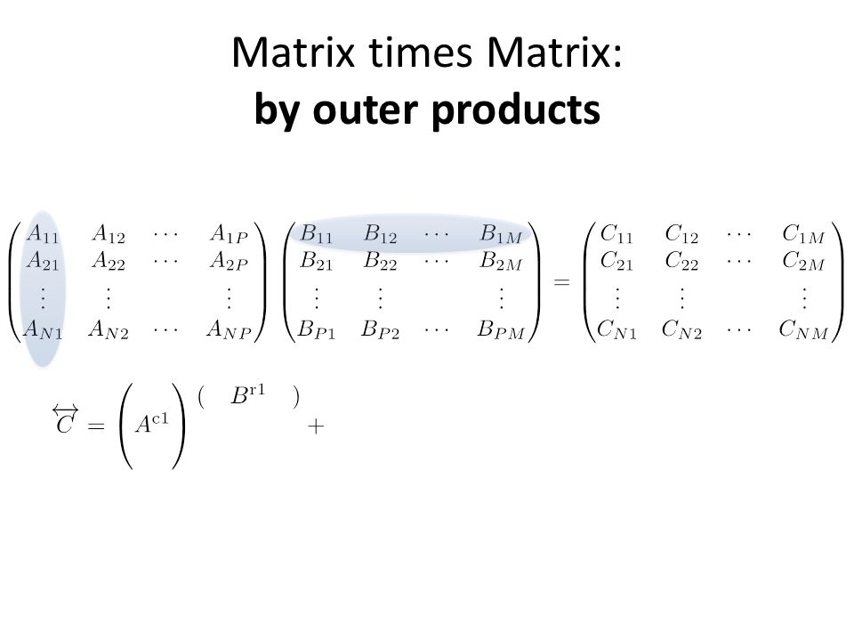
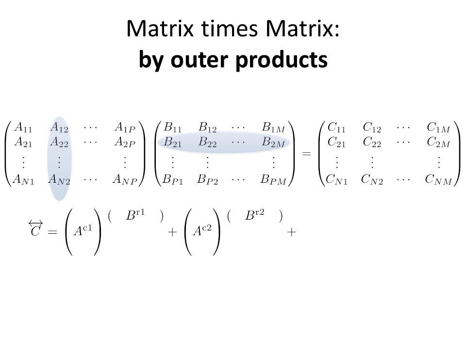
54. Matrix times Matrix: by outer products

57. C is a sum of outer products of the columns of A with the rows of B

58. Part 2: Matrix Properties (A few) special matrices Matrix transformations & the determinant Matrices & systems of algebraic equations

59. Special matrices: diagonal matrix This acts like scalar multiplication

60. Special matrices: identity matrix for all

61. Special matrices: inverse matrix Does the inverse always exist?

62. How does a matrix transform a square? (1,0) (0,1)

63. How does a matrix transform a square? (1,0) (0,1)

64. How does a matrix transform a square? (3,1) (0,2) (1,0) (0,1)

65. Geometric definition of the determinant: How does a matrix transform a square? (1,0) (0,1)

66. Example: solve the algebraic equation

68. 

69. Example of an underdetermined system Some non-zero vectors are sent to 0

70. Example of an underdetermined system

71. 

72. Some non-zero x are sent to 0 (the set of all x with Mx=0 are called the “nullspace” of M) This is because det(M)=0 so M is not invertible. (If det(M) isn’t 0, the only solution is x = 0) 

73. Part 3: Eigenvectors & eigenvalues

74. What do matrices do to vectors? (3,1) (0,2) (2,1)

75. Recall (3,5) (2,1)

76. What do matrices do to vectors? (3,5) The new vector is: 1) rotated 2) scaled (2,1)

77. Are there any special vectors that only get scaled?

78. Try (1,1)

79. Are there any special vectors that only get scaled? = (1,1)

80. Are there any special vectors that only get scaled? = (3,3) = (1,1)

81. Are there any special vectors that only get scaled? For this special vector, multiplying by M is like multiplying by a scalar. (1,1) is called an eigenvector of M 3 (the scaling factor) is called the eigenvalue associated with this eigenvector = (1,1) = (3,3)

82. Are there any other eigenvectors?

83. Yes! The easiest way to find is with MATLAB’s eig command. Exercise: verify that (-1.5, 1) is also an eigenvector of M.

84. Are there any other eigenvectors? Yes! The easiest way to find is with MATLAB’s eig command. Exercise: verify that (-1.5, 1) is also an eigenvector of M with eigenvalue 2 = -2 Note: eigenvectors are only defined up to a scale factor. – Conventions are either make e’s unit vectors, or make one of the elements 1

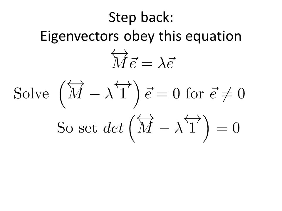
85. Step back: Eigenvectors obey this equation

88. This is called the characteristic equation for In general, for an N x N matrix, there are N eigenvectors

89. BREAK

90. Part 4: Examples (on blackboard) Principal Components Analysis (PCA) Single, linear differential equation Coupled differential equations

91. Part 5: Recap & Additional useful stuff Matrix diagonalization recap: transforming between original & eigenvector coordinates More special matrices & matrix properties Singular Value Decomposition (SVD)

92. Coupled differential equations Calculate the eigenvectors and eigenvalues. – Eigenvalues have typical form: The corresponding eigenvector component has dynamics:

93. Step 1: Find the eigenvalues and eigenvectors of M. Step 2: Decompose x into its eigenvector components Step 3: Stretch/scale each eigenvalue component Step 4: (solve for c and) transform back to original coordinates. Practical program for approaching equations coupled through a term Mx eig(M) in MATLAB

94. Step 1: Find the eigenvalues and eigenvectors of M. Step 2: Decompose x into its eigenvector components Step 3: Stretch/scale each eigenvalue component Step 4: (solve for c and) transform back to original coordinates. Practical program for approaching equations coupled through a term Mx

95. Step 1: Find the eigenvalues and eigenvectors of M. Step 2: Decompose x into its eigenvector components Step 3: Stretch/scale each eigenvalue component Step 4: (solve for c and) transform back to original coordinates. Practical program for approaching equations coupled through a term Mx

96. Step 1: Find the eigenvalues and eigenvectors of M. Step 2: Decompose x into its eigenvector components Step 3: Stretch/scale each eigenvalue component Step 4: (solve for c and) transform back to original coordinates. Practical program for approaching equations coupled through a term Mx

97. Step 1: Find the eigenvalues and eigenvectors of M. Step 2: Decompose x into its eigenvector components Step 3: Stretch/scale each eigenvalue component Step 4: (solve for c and) transform back to original coordinates. Practical program for approaching equations coupled through a term Mx

98. Step 1: Find the eigenvalues and eigenvectors of M. Step 2: Decompose x into its eigenvector components Step 3: Stretch/scale each eigenvalue component Step 4: (solve for c and) transform back to original coordinates. Practical program for approaching equations coupled through a term Mx

99. Where (step 1): MATLAB: Putting it all together…

100. Step 2: Transform into eigencoordinates Step 3: Scale by i along the i th eigencoordinate Step 4: Transform back to original coordinate system Putting it all together…

101. Left eigenvectors -The rows of E inverse are called the left eigenvectors because they satisfy E -1 M =  E -1. -Together with the eigenvalues, they determine how x is decomposed into each of its eigenvector components.

102. Matrix in eigencoordinate system Original Matrix Where: Putting it all together…

103. Note: M and Lambda look very different. Q: Are there any properties that are preserved between them? A: Yes, 2 very important ones: Matrix in eigencoordinate system Original Matrix Trace and Determinant 2. 1.

104. Special Matrices: Normal matrix Normal matrix: all eigenvectors are orthogonal  Can transform to eigencoordinates (“change basis”) with a simple rotation of the coordinate axes  E is a rotation (unitary or orthogonal) matrix, defined by: E Picture:

105. Special Matrices: Normal matrix Normal matrix: all eigenvectors are orthogonal  Can transform to eigencoordinates (“change basis”) with a simple rotation of the coordinate axes  E is a rotation (unitary or orthogonal) matrix, defined by: where if:then:

106. Special Matrices: Normal matrix Eigenvector decomposition in this case: Left and right eigenvectors are identical!

107. Symmetric Matrix: Special Matrices e.g. Covariance matrices, Hopfield network Properties: – Eigenvalues are real – Eigenvectors are orthogonal (i.e. it’s a normal matrix)

108. SVD: Decomposes matrix into outer products (e.g. of a neural/spatial mode and a temporal mode) t = 1 t = 2 t = T n = 1 n = 2 n = N

109. SVD: Decomposes matrix into outer products (e.g. of a neural/spatial mode and a temporal mode) n = 1 n = 2 n = N t = 1 t = 2 t = T

110. SVD: Decomposes matrix into outer products (e.g. of a neural/spatial mode and a temporal mode) Rows of V T are eigenvectors of M T M Columns of U are eigenvectors of MM T Note: the eigenvalues are the same for M T M and MM T

111. SVD: Decomposes matrix into outer products (e.g. of a neural/spatial mode and a temporal mode) Rows of V T are eigenvectors of M T M Columns of U are eigenvectors of MM T Thus, SVD pairs “spatial” patterns with associated “temporal” profiles through the outer product

112. The End