1. Seminar 3 Data requirements, limitations, and challenges: Inverse modeling of seed and seedling dispersal Likelihood Methods in Forest Ecology October 9 th – 20 th, 2006

2. Approaches to Estimation of Seed and Seedling Dispersal Functions Direct sampling around isolated trees ( David Greene) Develop mechanistic models with directly measurable parameters ( Ran Nathan) Inverse modeling using likelihood methods and neighborhood models (Eric Ribbens, Jim Clark, and a rapidly growing community of practitioners…)

3. The questions… l What are the shapes of the dispersal functions? l How does fecundity vary as a function of tree size? l What other factors determine the spatial distribution of seeds and seedlings around parent trees? - Wind direction (anisotropy) - Secondary dispersal - Density and distance - dependent seed predation and pathogens - Substrate conditions - Light levels

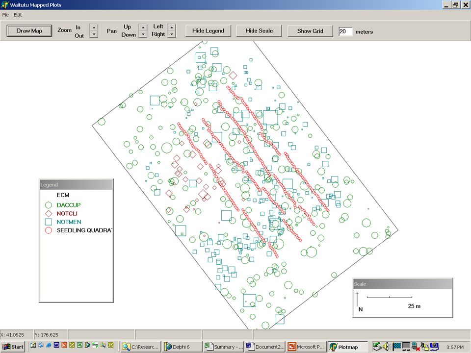
4. The basic approach: field methods l Map the distribution of potential parent trees within a stand l Sample the density of seeds or seedlings at mapped locations within the stand l Measure any additional features at the location of the seed traps or seedling quadrats

6. The Probability Model l Observations consist of counts l Assume the counts are either Poisson or Negative Binomial distributed l Poisson PDF: Where x = observed density (integer), and = predicted density (continuous)

7. Negative Binomial PDF “shape” of the PDF controlled by both the expected mean ( m ) and a “shape” parameter ( k ) As k varies, the distribution can vary from over- to under-dispersed (i.e. variance > or < mean) This is the notation for the gamma function…

8. The basic “scientific” model l Seed rain at a given location is the sum of the input of N parent trees, with the input from any given tree a function of the: - Size (typically DBH) and - Distance to the parent

9. How does total seed production vary with tree size? l Common assumption: seed production is a function of DBH 2 (following Ribbens et al. 1994) where  = 2, and STR = total standardized seed production of a 30 cm DBH tree Is this a reasonable assumption? Is it supported by either independent data or theory?

10. How does seed rain vary with distance from a parent tree? l Two basic classes of functions are commonly used*: - Monotonically declining (negative exponential): - Lognormal: *See Greene et al. (2004), J. Ecol. for a discussion…

11. One more trick… Normalizing the dispersal function [ g(dist)] so that STR is in meaningful units… Where  is the “arcwise” (i.e. 360 o ) integration of the dispersal function

12. Lognormal form: Exponential form: So, the basic scientific models…

13. The Scientific Models

14. Anisotropy: does direction matter? For the lognormal dispersal function: Incorporate effect of direction from source tree on modal dispersal distance 1 : 1 Staelens, J., L. Nachtergale, S. Luyssaert, and N. Lust. 2003. A model of wind-influenced leaf litterfall in a mixed hardwood forest. Canadian Journal of Forest Research.

15. Shape of the wind direction effect When would this matter? (just to increase goodness of fit and improve parameter estimation?)

16. Potential Dataset Limitations Censored data: not all parents are accounted for Insufficient variation in predicted values: parents are too uniformly distributed Two different populations treated as one: not all potential parents actually produce seeds Lack of independence: spatial autocorrelation among nearby samples

18. Effects of Search Radius

19. Sampling along the edge...

20. What if all of the trees are uniformly spaced? l This produces relatively similar neighborhoods for all observations… l Random vs. strategic sampling…

21. Goodness of Fit – Sites with Different Densities

22. What if all of the trees are the same size? Tradeoffs between STR and 

23. What if not all trees produce seed?

24. Can the data discriminate between different functions?

25. Beware of simplifying assumptions in your model...

26. Parameter Estimation – Varying 

27. What is the minimum size of a reproductive adult? l Most studies have arbitrarily assumed that all adults over a low minimum size (10 – 15 cm DBH) contribute seeds. l One approach – estimate the minimum (don’t assume it) How could we determine the effective minimum reproductive size?

28. Parent size and seedling production in a Puerto Rican rainforest Source: Uriarte et al. (2005) J. Ecology

29. Scaling reproductive output to tree size: Maximum likelihood parameter estimates Species  min. size (cm) Casearia arborea 0.1413.7 Dacryodes excelsa 0.51 NA Guarea guidonia 2.06 48.13 Inga laurina 2.38 16.39 Manilkara bidentata 0.01 44.04 Prestoea acuminata 0.15 13.89 Schefflera morototoni 3.22 9.61 Sloanea berteriana 1.70 11.06 Tabebuia heterophylla 0.01 20.93 Source: Uriarte, M., C. D. Canham, J. Thompson, J. K. Zimmerman, and N. Brokaw. 2005. Seedling recruitment in a hurricane-driven tropical forest: light limitation, density-dependence and the spatial distribution of parent trees. Journal of Ecology 93:291-304.

30. Should there be an “intercept” in the model? l Allowing for long-distance dispersal via a “bath” term: Where b is an average input of seeds even when there are no parents in the neighborhood…

31. For seedlings: does light influence germination? 0 < M(GLI) < 1 L opt Lhi = slope away from L opt Llo = slope to Lopt

32. Light Availability

33. Is there evidence of density dependence in seedling establishment? l Add yet another multiplier... C δ Conspecific seedling density DD Effect (0-1)

34. Negative Conspecific Density Dependence

35. Spatial autocorrelation

36. Dealing with spatial autocorrelation among observations… l Remember - the formula for calculating log-likelihood assumes that observations are independent… l We have been conditioned to assume that two observations taken at locations close together are likely to be not independent (a legacy of Stuart Hurlbert) l Moran’s I and other indices of spatial autocorrelation How do you determine whether this is true?

37. A critical distinction… l Remember – the issue is whether the residuals (the error terms in the probability model) are independent. NOT whether the raw observations are… If your scientific model “explains” why two nearby observations have similar values, then the fact that they are similar is NOT evidence of lack of independence*… *despite assertions to the contrary in some papers on the subject

38. So, examine your residuals for spatial autocorrelation Distance class (m) Moran’s I l A “best-case” species… Examples from a study of seedling recruitment in a New Zealand rainforest (data from Elaine Wright)

39. Another species… l A worse case… Distance class (m) Moran’s I

40. Causes and consequences of fine-scale spatial autocorrelation… l The causes are probably legion: - Many trees don’t produce seed in any given mast year, - Many factors can cluster input of seeds or survival of seedlings l The consequences are important but not fatal: - Generally very little bias in parameter estimates themselves, - But estimates of the variance of the parameters will be biased (low) Do the thought experiment or test this with real data – what would happen if you duplicated some observations in the dataset and then redid the analysis?