Download presentation
Presentation is loading. Please wait.

1
International Trade and Income Differences Michael E. Waugh

2
I. Introduction Standards of living between the richest and poorest countries differ by more than a factor of 30. The consensus is that physical and human capital accounts for only 50 percent of the variation in income per worker; the rest is productivity differences. Given this finding, a growing literature has attempted to understand how various frictions result in large differences in measured productivity across countries.

3
In this paper, the author develops a view of the frictions to trade between rich and poor countries by arguing that to reconcile bilateral trade volumes and price data within a standard gravity model, the trade frictions between rich and poor countries must be systematically asymmetric, with poor countries facing higher costs to export relative to rich countries. I then argue that these frictions to trade are quantitatively important to understanding why standards of living and measured total factor productivity between the richest and poorest countries differ by so much.

4
II. The Model Consider a world with N countries. Each country has two sectors: a tradable goods sector and a final goods sector. Within each country i, there is a measure of consumers Li. Each consumer has one unit of time supplied inelastically in the domestic labor market, and each is endowed with capital supplied to the domestic capital market. All variables are normalized relative to the labor endowment in country i.

5
A. Tradable Goods Sector II. The Model There is a continuum of tradable goods indexed by x ∈ [0,1]. Production function of tradable goods: Power terms,, are common to all countries.

6
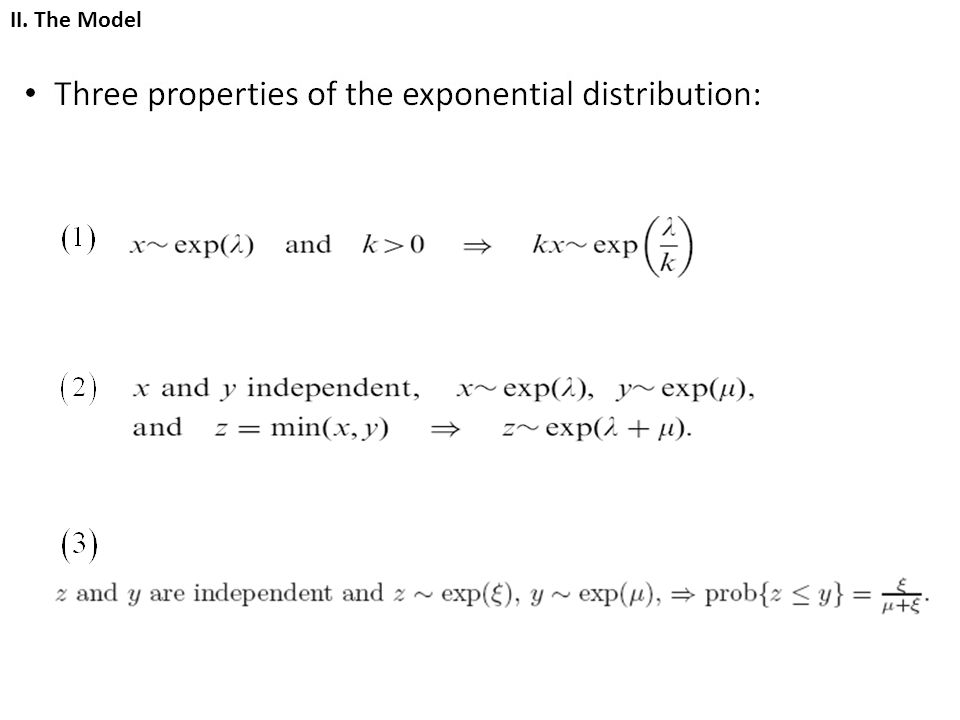
— Production Technologies In Eaton and Kortum (2002), the inverses of TFP levels are modeled as random variables, independent across goods, with a common density. As in Alvarez and Lucas (2007), here we assume that is distributed independently and exponentially with parameter differing across countries. That is, All firms in country i have access to the technology for any good x with the efficiency level. II. The Model
, here we assume that is distributed independently and exponentially with parameter differing across countries. That is, All firms in country i have access to the technology for any good x with the efficiency level. II. The Model.")
7
These draws are amplified in percentage terms by the parameter. The random variables good-level productivity then have a Type II extreme value distribution (Frechet distribution). governs each country’s average productivity level. controls the dispersion of efficiency levels. II. The Model
. governs each country’s average productivity level. controls the dispersion of efficiency levels. II. The Model.")
8
— Aggregated Tradable Goods II. The Model Spence – Dixit – Stiglitz (SDS) form:
 form:")
9
B. Final Goods Sector II. The Model Production function of final goods sector:

10
C. Trade Costs II. The Model

11
D. Equilibrium II. The Model

13
III. Trade Data, Price Data, and Model ⇒ Asymmetric Trade Costs A.Trade Data O.1. Home bias for both rich and poor countries. The important observation is that there is little variation in the Xiis relative to a country’s income per worker. Rich countries purchase slightly more from home than poor countries, but the difference in magnitude is small.

14
O.2. Systematic correlation between bilateral trade shares and relative level of development. The values encompassing poor countries’ imports from rich countries are large relative to that of rich countries’ imports from poor countries. B. Price Data O.3. Aggregate tradable goods prices are similar between rich and poor countries.

15
C. The Implications of Trade Data, Price Data, for Trade Costs

16
A. Common Elements to Both Examples IV. Modeling Asymmetry: Some Examples

17
1) Implications for Prices: 2) Implications for Income Differences: B. Example 1: Export Effects
 Implications for Prices: 2) Implications for Income Differences: B. Example 1: Export Effects")
18
1) Implications for Prices: 2) Implications for Income Differences: C. Example 2: Import Effects
 Implications for Prices: 2) Implications for Income Differences: C. Example 2: Import Effects")
19
A. Benchmark Approach V. Estimating Technology and Trade Costs from Trade Data

20
B. Alternative Approach

21
C. Recovering Technology

22
A. Estimation Approach B. Disaggregated Price Data C. A Benchmark Estimate of VI. Estimating

23
VII. Measurement and Common Parameter Values A. Measuring Income PerWorker B. Factor Shares C. Capital, Labor, and Distance Data

24
VIII. Estimation Results A. Benchmark Results

26
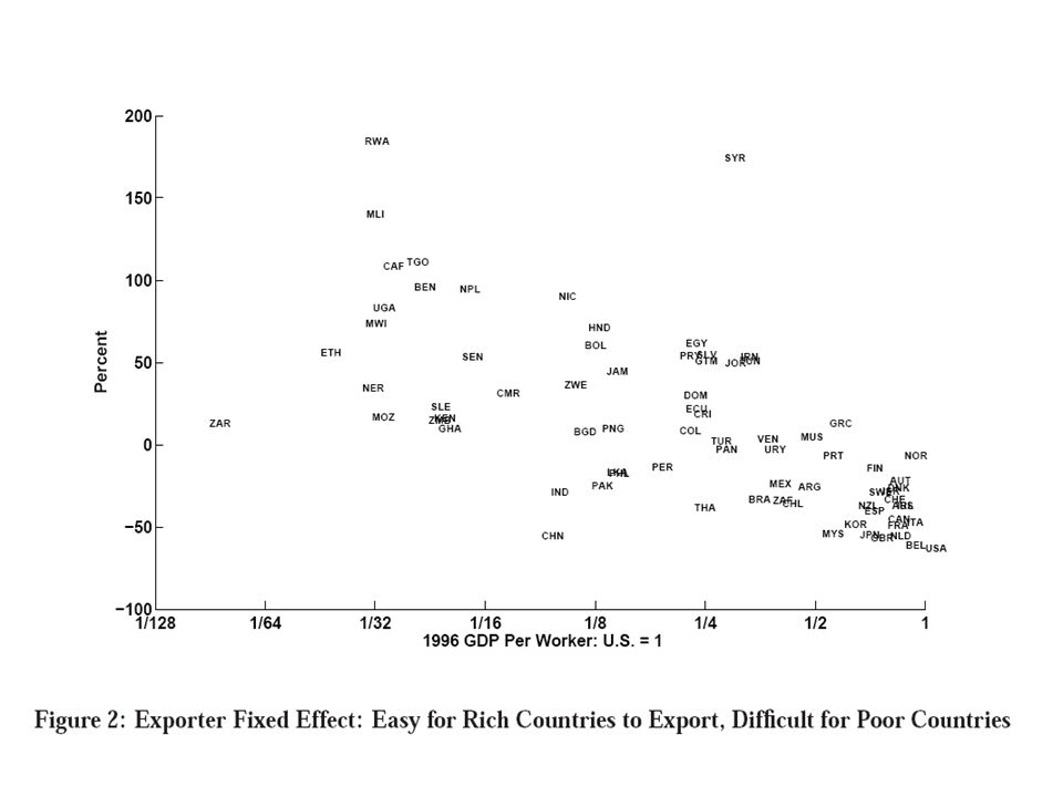
B. A Comparison to the Model with Importer Fixed Effects

27
IX. The Quantitative Implications of the Estimated Model A. The Benchmark Model

29
B. The Implications of the Estimated Model with Importer Fixed Effects

30
C. A Brief Discussion To clarify the forces driving these outcomes, recall that the model with importer fixed effects reconciles the fact that the United States imports more from Japan than Senegal by making unit costs of production (on average) lower in Japan than in Senegal. In contrast, the model with exporter fixed effects reconciles the differences in the United States’ import share from Japan relative to Senegal by manipulating each country’s export cost. The model reconciles the similarities in Japan’s and Senegal’s import share from the United States with similar unit costs of production.
 lower in Japan than in Senegal. In contrast, the model with exporter fixed effects reconciles the differences in the United States’ import share from Japan relative to Senegal by manipulating each country’s export cost. The model reconciles the similarities in Japan’s and Senegal’s import share from the United States with similar unit costs of production..")
31
X. How Do Trade Costs Affect Income Differences? A. Eliminating Asymmetries in Trade Costs Reduces Income Differences

32
B. On The Mechanics Behind Reductions in Income Differences

33
XI. Robustness Checks and Alternative Evidence A. Price Data: A Robustness Check

34
B. Alternative Evidence on Asymmetric Trade Costs

35
C. Evidence from Trade Liberalizations

36
XII. Conclusion This paper have argued that systematically asymmetric trade frictions are necessary to reconcile both price and quantity data in a standard model of international trade. Furthermore, these asymmetries are quantitatively important to understanding cross-country income differences. The author suggests two routes to further understand this puzzle that are complements rather than substitutes. 1)One is better theory, i.e., some of these frictions may be reduced-form representations of equilibrium responses to the fundamen-tals faced by agents; e.g., the model of Fieler (2007) with nonhomothetic preferences is an example. 2)Analternative route is better measurement. Measuring bilateral trade flows in value added, exploiting disaggregate trade flows, and disaggregate measures of tariff and non-tariff barriers are all possible avenues for future research as well.
One is better theory, i.e., some of these frictions may be reduced-form representations of equilibrium responses to the fundamen-tals faced by agents; e.g., the model of Fieler (2007) with nonhomothetic preferences is an example. 2)Analternative route is better measurement. Measuring bilateral trade flows in value added, exploiting disaggregate trade flows, and disaggregate measures of tariff and non-tariff barriers are all possible avenues for future research as well..")
Similar presentations


>")


The Case for Trade 1) A country has a.>")


