1. Waiting Lines and Queuing Theory Models
Chapter 2
Waiting Lines and Queuing Theory Models

2. Learning Objectives Students will be able to:
Describe the trade-off curves for cost-of-waiting time and cost-of-service.
Explain the three parts of a queuing system: the calling population, the queue itself, and the service facility.
Explain the basic queuing system configurations.
Describe the assumptions of the common queuing system models.
Analyze a variety of operating characteristics of waiting lines.

3. Chapter Outline
5.1 Introduction. 5.2 Waiting Line Costs. 5.3 Characteristics of a Queuing System. 5.4 Single-Channel Queuing Model with Poisson Arrivals and Exponential Service Times (M/M/1). 5.5 Multi-Channel Queuing Model with Poisson Arrivals and Exponential service Times (M/M/m). 5.6 Constant Service Time Model (M/D/1). 5.7 Finite Population Model (M/M/1 with Finite Source). 5.8 Some General Operating Characteristics Relationships. 5.9 More Complex Queuing Models and the Use of Simulation.

4. 1. Introduction
Queuing theory is one of the most widely used quantitative analysis techniques.
The three basic components are:
Arrivals,
Service facilities,
Actual waiting line.
Waiting line problems are centered on the questions of finding the ideal level of services that the firm should provide.

5. 1. Introduction (Cont’d.)
- Supermarkets, decides how many cash register check out positions opened. - Gasoline stations, the number of pumps opened. - Manufacturing plants, the optimal number of mechanics to have on duty for repair. - Banks, the number of teller windows to keep open to serve customers in various hours of a day.

6. 2. Waiting Line Costs Queuing analysis includes:
Determining the best level of service.
Analyzing the trade-off between cost of providing service and cost of waiting time.
Most managers want queues that are short enough so that customers do not become unhappy.
One means of evaluating a service facility is to look at a total expected cost, which is the sum of expected service cost plus expected waiting cost, see the following figure:

7. Queuing Costs and Service Levels
Total Expected Cost
Cost of Providing
Service
Cost of Waiting Time
Optimal Service Level

8. Three Rivers Shipping Co. Example
The superintendent at Three Rivers Shipping Company wants to determine the optimal number of stevedores to employ each shift.
Number of Stevedores Working 1 2 3 4
(a) Avg. number of ships arriving per shift 5
(b) Average waiting time per ship to be unloaded (hours) 7 4 3 2
(c) Total ship hours lost per shift (a × b) 35 20 15 10
(d) Estimated cost per hour of idle ship time
$1,000
(e) Value of ship’s lost time (c × d)
$35,000
$20,000
$15,000
$10,000
(f) Stevedore teams salary
$6,000
$12,000
$18,000
$24,000
(g) Total expected cost (e+f)
$41,000
$32,000
$33,000
$34,000

9. 3. Characteristics of a Queuing System
Arrival Characteristics:
Size of the calling population.
Pattern of arrivals.
Behavior of arrivals.
Waiting Line Characteristics:
Queue length.
Queue discipline.
Service Facility Characteristics:
Configuration of the queuing system.
Service time distribution.

10. Arrival Characteristics of a Queuing System
Calling Population:
Unlimited (infinite).
Limited (finite).
Arrival Pattern:
Randomly.
Poisson Distribution.

11. Arrival Characteristics: Poisson Distribution
For X = 0, 1, 2, 3, 4, …
.00
.05
.10
.15
.20
.25
.30
.35 1 2 3 4 5 6 7 8 9 10 X
P(X)
P(X),  = 2
.00
.05
.10
.15
.20
.25
.30 1 2 3 4 5 6 7 8 9 10 11 X
P(X)
P(X),  = 4

12. Arrival Characteristics of a Queuing System (continued)
Behavior of arrivals:
Join the queue, wait till served, and do not switch between lines.
Balk; refuse to join the line.
Renege (Withdraw); enter the queue, but then leave without completing the transaction.

13. Waiting Line Characteristics of a Queuing System
Length of the queue:
Limited.
Unlimited.
Service priority/Queue discipline:
First In First Out (FIFO).
Other.

14. Service Facility Characteristics
Configuration of the queuing system:
Number of channels (servers):
Single.
Multiple.
Number of phases in service system (customer stations):
Single (1 stop).
Multiple (2+ stops).
Service time distribution:
Exponential.
Other.

15. Service Characteristics: Queuing System Configurations
Single Channel, Single Phase
Queue
Service
facility
arrivals
Departure after Service
A bank which has only one open teller.
Facility 1 2
Single Channel, Multi-Phase
Queue
Service Facility
arrivals
Departure after Service

16. Service Characteristics: Queuing System Configurations
facility 1
facility 2
facility 3
Multi-Channel, Single Phase System
Queue
arrivals
Departure after Service
Multi-Channel,
Multiphase System
Queue
Type 1 Service Facility
Type 2 Service Facility
arrivals
Departure after Service

17. Service Characteristics of a Queuing System
Service Time Patterns:
Exponential probability distribution.
Other distributions.

18. Service Time Characteristics: Exponential Distribution
Probability
Average Service Time of 20 Minutes
Average Service Time of 1 Hour
Service Time (Minutes), X

19. Identifying Models Using Kendall Notation
The basic three-symbol Kendall notation:
Arrival Service Time Number of Service
Distribution Distribution Channels Open
Where:
M = Poisson distribution for the number of occurrences (or exponential times).
D = Constant (deterministic rate).
G = General distribution with mean and variance known.
M/M/1
A Single channel model with Poisson arrivals and exponential service times.
M/M/2
When a second channel is added

20. Identifying Models Using Kendall Notation (Cont’d.)
If there are m distinct service channels in the queuing system with Poisson arrivals and exponential service times, the Kendall notations will be:
A three channel system with poisson arrivals and constant service time is:
A four-channel system with Poisson arrivals and service times that are normally distributed would be:
M / M / m
M / D / 3
M / G / 4

21. Assumptions of the Model:
4. Single-Channel Queuing Model with Poisson Arrivals and Exponential Service Times (M / M/ 1)
Assumptions of the Model:
1. Queue discipline: FIFO. 2. No balking or reneging. 3. Arrivals: Poisson distributed. 4. Independent arrivals; constant rate over time. 5. Service times: exponential, average known. 6. Average service rate > average arrival rate.

22. M/M/1 Single channel

23. Operating Characteristics of Queuing Systems
Average number of customers in the system (L).
Average time each customer spends in the system (W).
Average length of the queue (Lq).
Average time each customer spends waiting in the queue (Wq).
Utilization factor for the system (ρ).
Probability that the service facility will be idle (P○).
Probability that the number of customers in the system (n) is greater than k, (Pn > k).

24. Queuing Equations
ג = mean number of arrivals per time period,
μ = mean number of customers served per time period.
7. Probability that the number of customers in the system (n) is > k,

25. Arnold’s Muffler Shop Case
Assume you are planning a car wash to raise money for a local charity.
You anticipate the cars arriving in a single line and being serviced by one team of washers.
Based on historical data, you believe cars will arrive every 30 minutes, and the team can wash a car in about 20 minutes.
The arrival rates follow a Poisson distribution and the service rates are exponentially distributed.
What are the operating characteristics for this system?

26. Arnold’s Muffler Shop Case
Assume you are planning a car wash to raise money for a local charity.
You anticipate the cars arriving in a single line and being serviced by one team of washers.
Based on historical data, you believe cars will arrive every 30 minutes, and the team can wash a car in about 20 minutes.
The arrival rates follow a Poisson distribution and the service rates are exponentially distributed.
What are the operating characteristics for this system? 26

27. = 2 cars arriving per hour
Arnold’s Muffler Shop Case
Assume you are planning a car wash to raise money for a local charity.
You anticipate the cars arriving in a single line and being serviced by one team of washers.
Based on historical data, you believe cars will arrive every 30 minutes, and the team can wash a car in about 20 minutes.
The arrival rates follow a Poisson distribution and the service rates are exponentially distributed.
What are the operating characteristics for this system? 
= 2 cars arriving per hour
μ = 3 cars serviced per hour

28. Car Wash Example: Operating Characteristics
= 2 cars arriving per hour,
μ = 3 cars serviced per hour
L = ? cars in the system on average
W= ? hours that an average car spends in the system
Lq= ? cars waiting on average
Wq= ? hours is average wait in line
ρ = ? percent of time car washers are busy
P0= ? probability that there are 0 cars in the system
Let’s work through a simple example together…. Assume you are the troop leader of a girl scout troop who is planning a car wash to raise money. You want to have a good understanding of what the lines and service times will be before the big ‘wash-o-ton’ on Saturday. You have also promised the local gas station where the event will occur that cars won’t be backed-up into their regular customer parking. You anticipate the cars arriving in a single line and being serviced by one team of washers (the rest of the girls are holding up poster boards enticing additional business).
Being the competitive troop leader that you are and wanting to surpass the other troops in dollars raised, you having been spying on similar car wash schemes over the course of the last 3 months. Based on your observations you have determined that cars arrive every 30 minutes, or 2 per hour and you can wash a car in about 20 minutes or 3 per hour. (Your troop’s average age is 7 years old, so expedience is not your strong suit!) The arrival rates do follow a Poisson distribution and the service rates are exponentially distributed.
You are interested in determining the number of cars in the system and the amount of time the car spends in the system. You know people hate to wait and you fear they may go elsewhere if the system is back logged….

29. Car Wash Example: Operating Characteristics Solution
L = = 2/(3-2) cars in the system on average
W= = 1/(3-2) hour that an average car spends in the
system
Lq= = 22/[3(3-2)] cars waiting on average
Wq = = 2/[3(3-2)] hours is average wait ρ = = 2/ percent of time washers are busy
P0 = =1 – (2/3) probability that there are 0 cars in
the system
Using your newly acquired knowledge gained from your Management Science course you determine that there will be an average of 2 cars in the system. This will make the gas station owner happy because his lot won’t be overrun by the girl scouts’ customers!
The average car will spend 1 hour in the system… WOW you might be in trouble here! If it takes 20 minutes to was a car that means there will be an average of 40 minutes that someone will be waiting – this is also shown a Wq = .67 hours (note that .67 hours = 40.2 minutes). You may need to come up with a good skit to entertain the waiting customers – or maybe set up a booth to sell cookies !~
On average their will be 1.33 cars waiting to be serviced – GREAT chance to sell those cookies!
The probability the system will be busy is .67 which implies that 67% of the time the girls will be busy… well, never say you didn’t make them earn their money!! Now what will you do with a bunch of 7 year olds during the 33% of the time that there are no cars waiting to be washed???

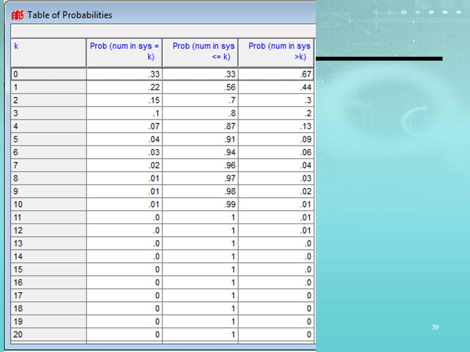
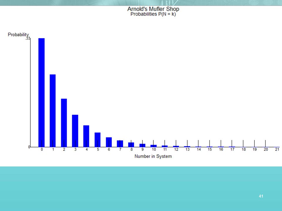
30. Probability of More Than k Cars in the System:
k Pn > k
0.444
0.296
0.198
0.132
0.088
0.058
0.039
Equal to 1-P0 =

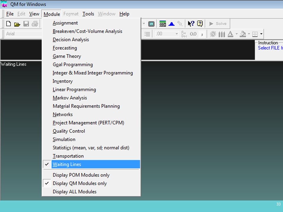
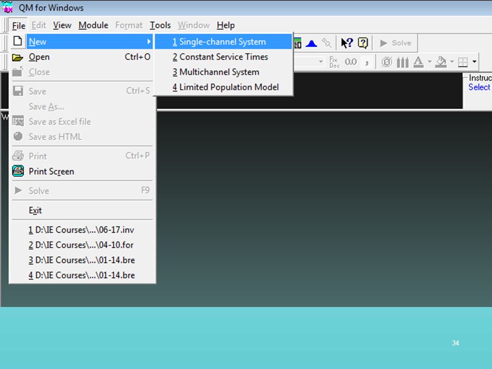
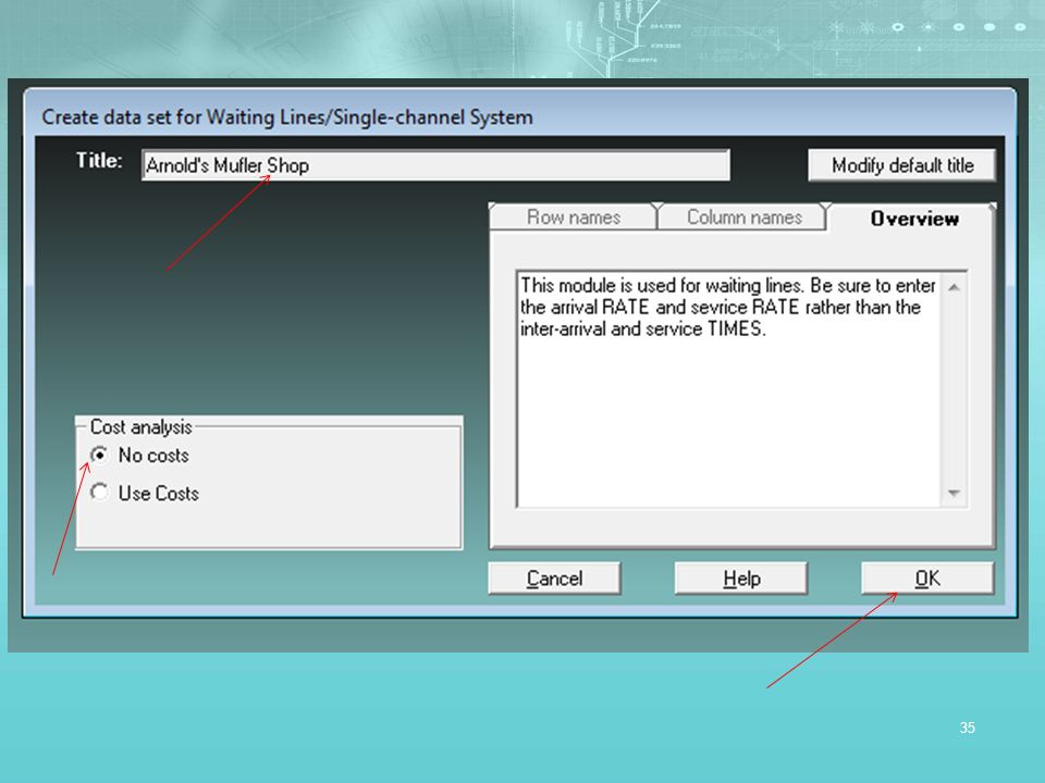
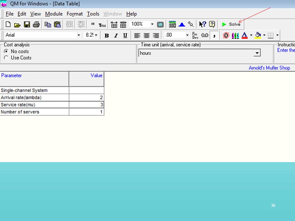
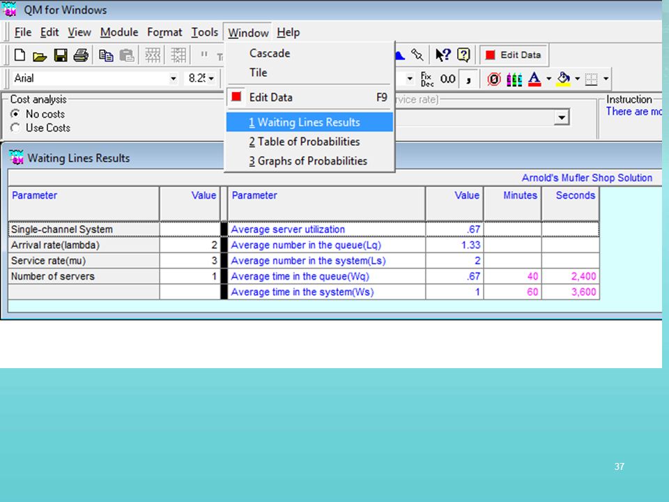
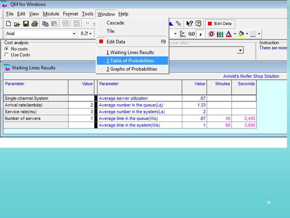
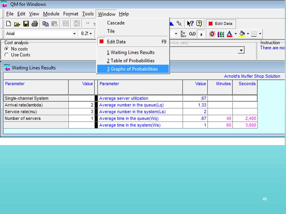
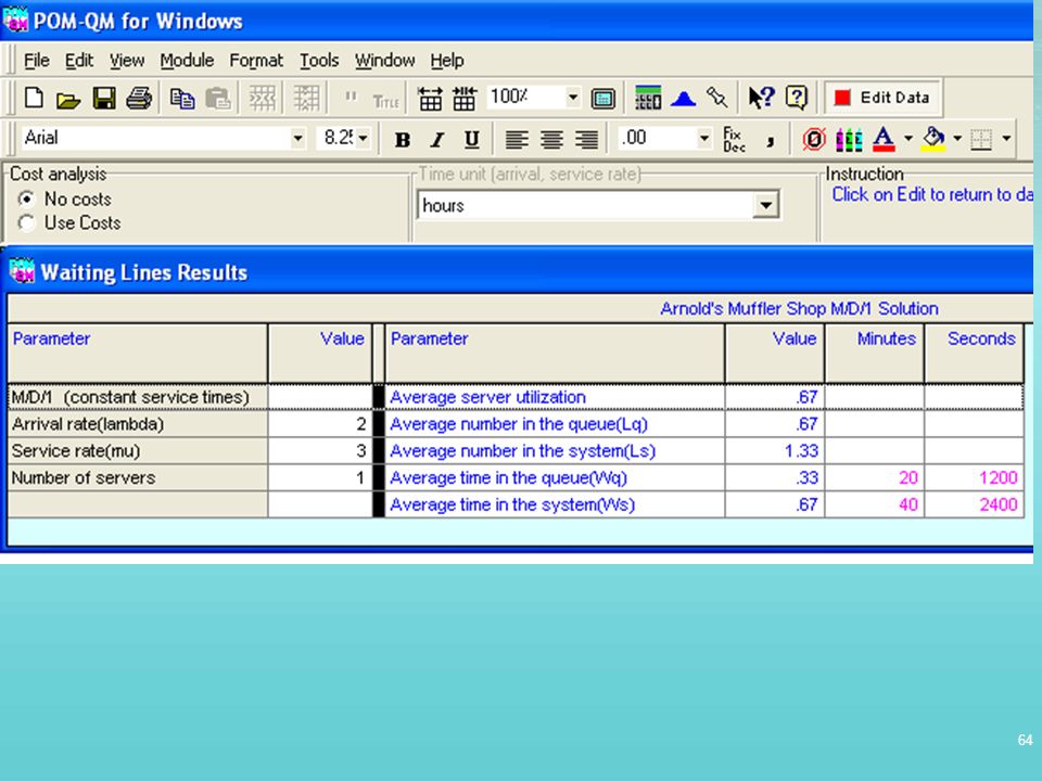
31. Solution Using QM for Windows
Lab Exercise:
Solution Using QM for Windows
Solve the Arnold’s Muffler Shop Example using Excel and QM for Windows.
To be continued.

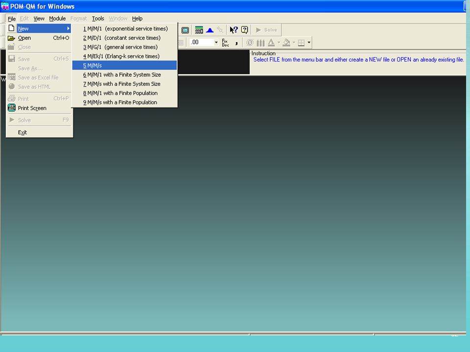
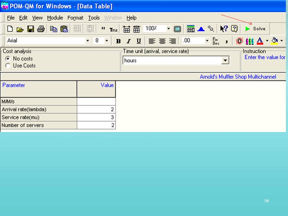
32. Using QM for Windows

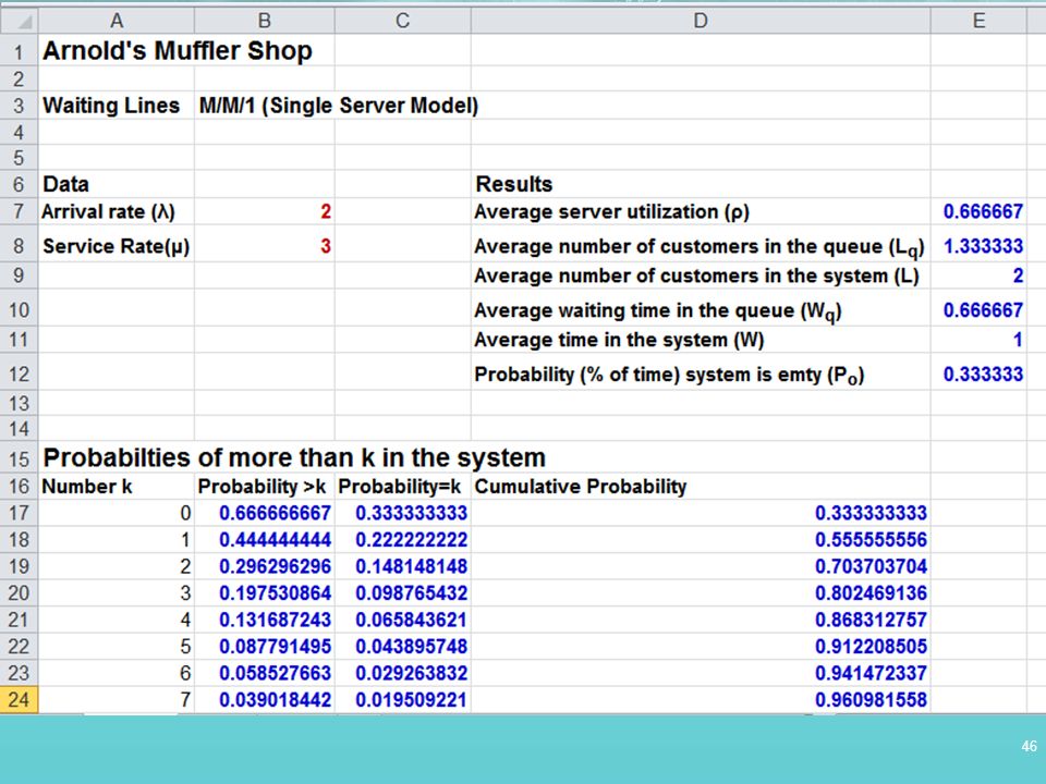
42. Solving Using Excel
ρ =
Average server utilization

43. L = , W= , Lq= , Wq = , ρ = , P0 = =B7/B8 =B7^2/(B8*B8-B7))
=1 – E7

44. Results:

45. , Pn = k = Pn>k-1 - Pn>k , k=1,2,…
Pn>0 = 1- Po ,
, Pn = k = Pn>k-1 - Pn>k , k=1,2,…
=1-E =E =C17
=(B7/B8)^(A18+1) =B17-B =C17+C18
=(B7/B8)^(A19+1) =B18-B =C18+C19
=(B7/B8)^(A20+1) =B19-B =C19+C20
=(B7/B8)^(A21+1) =B20-B =C20+C21
=(B7/B8)^(A22+1) =B21-B =C21+C22
=(B7/B8)^(A23+1) =B22-B =C22+C23
=(B7/B8)^(A24+1) =B23-B =C23+C24

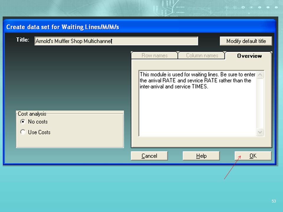
47. 5. Multichannel Queuing Model with Poisson Arrivals and Exponential Service Times (M/M/m)
A good example for the multichannel model is the super market, where you have more than one channel
M/M/m

48. 5. Multichannel Queuing Model with Poisson Arrivals and Exponential Service Times (M/M/m)
Equations for the Multichannel Queuing Model:
m = number of channels open.
1. Probability there are no customers in the system: l m n P - ç è æ + ú û ù ê ë é ø ö = å ! 1
>
for
2. Average number of customers in the system: ( ) m l lm + - è æ = P ! 1 L 2 ø ö

49. Equations for the Multichannel Queuing Model (Cont’d.)
3. The average time a customer spends in the system, l L = W m l L - = q
4. The average number of customers in line waiting,
5. The average time a customer spends in the queue waiting for service, q l m L W = - 1 m l r =
6. The utilization rate,

50. Arnold’s Muffler Shop Revisited
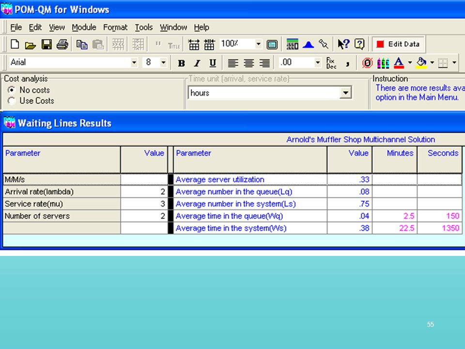
Should you have 2 teams of car washers? 
= 2 cars/ hr
u = 3 cars/ hr , m =2 1
= = 0.5 2
P0 = / 1! + 2
= = 0.75 4
L =
W = = 3 = 22.5 minutes
Lq = 0.75 – = =
Wq = = hour = 2.5 minutes 2

51. Lab Exercise (Cont’d.) Solution Using QM for Windows
2. Solve the Arnold’s Muffler Shop with 2 teams of car washers Example using Excel QM.
To be continued.

56. 6. Constant Service Time Model (M/D/1)2 L q - =
1. Average length of the queue,
2. Average waiting time in the queue,
3. Average number of customers in the queue,
4. Average time in the system,
(14-20) ( ) l m 2 W q - =
(14-21)
Lq and Wq are halved w.r.t. M/M/1 m l L + = q
(14-22) m 1 W + = q
(14-23)

57. Car Wash Example: M/D/1

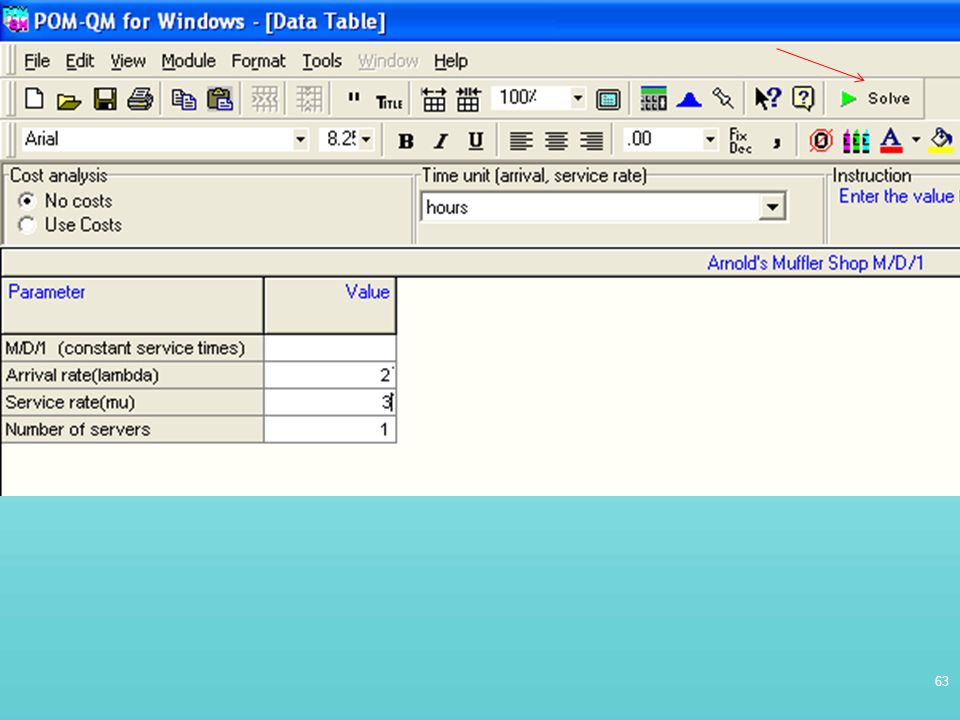
58. Car Wash Example: M/D/1
Your charity is considering purchasing an automatic car wash system.
Cars will continue to arrive according to a Poisson distribution, with 2 cars arriving every hour.
However, the service time will now be constant with a rate of 3 cars per hour.
- Compare the operating characteristics of this model with your previous models.

59. Car Wash Example: Operating Characteristics M/D/1
M/D/1 M/M/1 4
2(3) (3-2) 2 3
Lq = =
4 cars 3
2 hour
2 cars
1 hour 2
2(3)(3-2) 1 3
Wq = =
Both Lq and Wq are reduced by 50%! 4 3
L = = 2 3
W = =

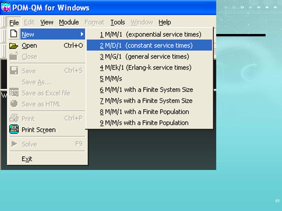
60. Lab Exercise (Cont’d.)
3. Solve the Arnold’s Muffler Shop M/D/1 Example using Excel QM or QM for Windows.

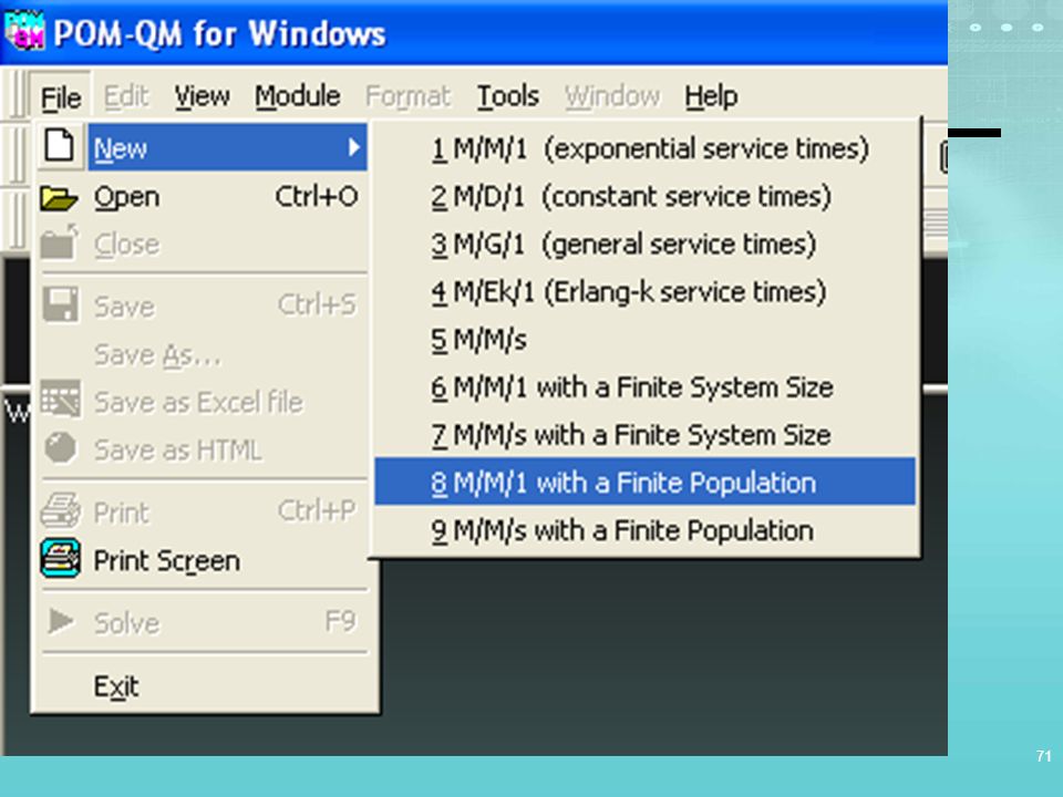
65. 7. Finite Population Model (M/M/1 with Finite Source)
Equations for the Finite Population Model
1. The probability that the system is empty: )! ( ! 1 P n N ø ö ç è æ - = å m l
N = size of the population
2. Average length of the queue: ( ) q 1 L P N - ø ö ç è æ + = l m
3. Average number of customers (units) in the system: ( ) 1 L P q - + =

66. ( ) ( ) ! Equations for the Finite Population Model (Cont’d.) W L N -
4. Average waiting time in the queue: ( ) q W L N - = l
5. Average time in the system: 1 W q + = m
6. Probability of n units in the system: ( ) n ! P N)
P(n, N ø ö ç è æ - = m l
For n = 0, 1, 2, ……., N

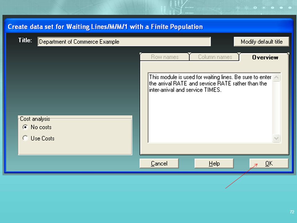
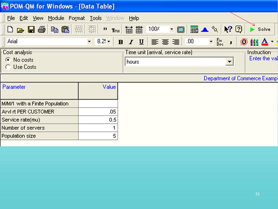
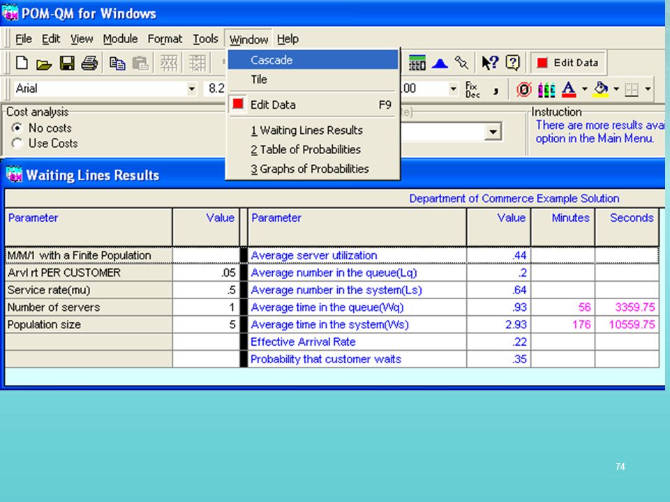
67. Department of Commerce Example:
The Department of Commerce has 5 printers that each need repair after about 20 hours of work.
Breakdowns follow a Poisson distribution.
The technician can service a printer in an average of about 2 hours, following an exponential distribution.
Determine the operating characteristics for this model.

68. Department of Commerce Example:

69. Operating Characteristics M/M/1 Finite source
= 1/20 = 0.05 printer/ hr,
u = ½ = 0.50 printer/ hr,
N = 5 1 5!
(5-n)! ∑ n
n=0 5
= 0.564
P0 =
0.05
(1-Po) = 5 – 4.8 = 0.2
Lq =
5 -
L = ( ) = 0.64 printer
0.2
(5-0.64)(0.05)
= 0.91 hour
Wq =
W = = 2.91 hours
0.50

70. Lab Exercise (Cont’d.).
4. Solve the Department of Commerce Example using Excel QM or QM for Windows.

75. 8. Some General Operating Characteristic Relationships
After reaching a steady state, certain relationships exist among specific operating characteristics.
A steady state condition exists when a queuing system is in its normal stabilized operating conditions, usually after an initial or transient state that may occur (e.g. having customers waiting at the door when a business opens in the morning). Both the arrival rate and the service rate should be stable in this state.

76. Little’s Flow Equations:
(14-30)
(14-31)
(14-32)
This is important because for certain queuing models, one of these may be much easier to determine than the others.
These are applicable to all of the queuing systems discussed in this chapter except the finite population model.

77. 9. More Complex Queuing Models and the Use of Simulation
Computer simulation is used to handle many real-world queuing applications that are complex.
Simulation allows:
Analysis of controllable factors.
Approximation of the actual service system.