Download presentation
Presentation is loading. Please wait.

1
Space-Efficient Online Computation of Quantile Summaries SIGMOD 01 Michael Greenwald & Sanjeev Khanna Presented by ellery

2
Outline Introduction The summary data structure Operation and algorithm Tree representation Analysis and experimental result Conclusion

3
Introduction Space-efficient computation of quantile summaries of very large data sets in a single pass. Quantile queries: Given a quantile, , return the value whose rank is N

4
t0t0 t1t1 t2t2 t3t3 t4t4 t5t5 t6t6 t7t7 t8t8 t9t9 t 10 t 11 t 12 t 13 t 14 t 15 121011101 119678 4523 sorting 1, 2, 3, 4, 5, 6, 7, 8, 9, 10, 10, 10, 11, 11, 11, 12 N = 16 0.5 quantile returns element ranked 8 ( 0.5*16) which is 8 0.75 quantile returns element ranked 12 (0.75*16) which is 10
 which is quantile returns element ranked 12 (0.75*16) which is 10")
5
Requirements Explicit & tunable a priori guarantees on the precision of the approximation As small a memory footprint as possible Online: Single pass over the data Data Independent Performance: guarantees should be unaffected by arrival order, distribution of values, or cardinality of observations. Data Independent Setup: no a priori knowledge required about data set (size, range, distribution, order).
..")
6
ε- approximate A quantile summary for a data sequence is ε- approximate if, for any given rank r, it returns a value whose rank r’ is guaranteed to be within the interval [r -εN, r + εN ] Example : A data stream with 100 elements, 0.5 – quantile with ε= 0.1 returns a value v. The true rank of v is within [40,60]
![ε- approximate A quantile summary for a data sequence is ε- approximate if, for any given rank r, it returns a value whose rank r’ is guaranteed to be within the interval [r -εN, r + εN ] Example : A data stream with 100 elements, 0.5 – quantile with ε= 0.1 returns a value v.](http://images.slideplayer.com/26/8847810/slides/slide_6.jpg "The true rank of v is within [40,60].")
7
The Summary Data Structure Let r min (v) and r max (v) denote the lower and upper bounds on the rank of v Each tuple ti = (v i, g i,Δ i )
 and r max (v) denote the lower and upper bounds on the rank of v Each tuple ti = (v i, g i,Δ i )")
8
Example .01, N=1750 192 {15,2} 201 {28,7} 204 {10,1} [501,503] [529,536] [539,540]
![Example .01, N= {15,2} 201 {28,7} 204 {10,1} [501,503] [529,536] [539,540]](http://images.slideplayer.com/26/8847810/slides/slide_8.jpg "Example .01, N= {15,2} 201 {28,7} 204 {10,1} [501,503] [529,536] [539,540]")
9
Query Sketch S is ε- approximate, That is for each ψ (0,1], there is a (v i, r min ( v i ), r max ( v i ) ) in S such that v i is our answer for ψ-quantile
![Query Sketch S is ε- approximate, That is for each ψ (0,1], there is a (v i, r min ( v i ), r max ( v i ) ) in S such that v i is our answer for ψ-quantile](http://images.slideplayer.com/26/8847810/slides/slide_9.jpg "Query Sketch S is ε- approximate, That is for each ψ (0,1], there is a (v i, r min ( v i ), r max ( v i ) ) in S such that v i is our answer for ψ-quantile")
10
Corollary If at any time n, the summary S(n) satisfies the property that then we can answer any ψ-quantile query to within an εn precision.
 satisfies the property that then we can answer any ψ-quantile query to within an εn precision.")
11
Overview of Summary Data Structure Quantile =.29? Compute r and choose best v i 192 [501,503] {15,2} 201 [529,536] {28,7} .01, N=1800 204 [539,540] { 10,1 } =.29 r = N = 522

12
Overview of Summary Data Structure If (r max (v i+1 ) - r min (v i )) ≦ 2 N, then - approximate summary. Our goal: always maintain this property. Tuple formulation of this rule: g i + I ≦ 2 N 192 [ 501,503 ] {15,2} 201 [529,536] {28,7} .01, N=1800 204 [539,540] {10,1} 2 N=36

13
Overview of Summary Data Structure Goal: always maintain -approximate summary (r max (v i+1 ) - r min (v i )) = (g i + I ) ≦ 2 N Insert new observations into summary 192 [501,503] {15,2} 201 [529,536] {28,7} .01, N=1800 204 [539,540] {10,1} 197 2 N=36
![Overview of Summary Data Structure Goal: always maintain -approximate summary (r max (v i+1 ) - r min (v i )) = (g i + I ) ≦ 2 N Insert new observations into summary 192 [501,503] {15,2} 201 [529,536] {28,7} .01, N= [539,540] {10,1} N=36](http://images.slideplayer.com/26/8847810/slides/slide_13.jpg "Overview of Summary Data Structure Goal: always maintain -approximate summary (r max (v i+1 ) - r min (v i )) = (g i + I ) ≦ 2 N Insert new observations into summary 192 [501,503] {15,2} 201 [529,536] {28,7} .01, N= [539,540] {10,1} N=36")
14
Overview of Summary Data Structure 192 [501,503] {15,2} 201 [529,536] {28,7} .01, N=1800 204 [539,540] {10,1} 197 [502,536] 2 N=36 Goal: always maintain -approximate summary (r max (v i+1 ) - r min (v i )) = (g i + I ) ≦ 2 N Insert new observations into summary
![Overview of Summary Data Structure 192 [501,503] {15,2} 201 [529,536] {28,7} .01, N= [539,540] {10,1} 197 [502,536] 2 N=36 Goal: always maintain -approximate summary (r max (v i+1 ) - r min (v i )) = (g i + I ) ≦ 2 N Insert new observations into summary](http://images.slideplayer.com/26/8847810/slides/slide_14.jpg "Overview of Summary Data Structure 192 [501,503] {15,2} 201 [529,536] {28,7} .01, N= [539,540] {10,1} 197 [502,536] 2 N=36 Goal: always maintain -approximate summary (r max (v i+1 ) - r min (v i )) = (g i + I ) ≦ 2 N Insert new observations into summary")
15
Overview of Summary Data Structure Goal: always maintain -approximate summary (r max (v i+1 ) - r min (v i )) = (g i + I ) ≦ 2 N Insert new observations into summary Insert tuple before the ith tuple. g new = 1; new = g i + I - 1; 192 [501,503] {15,2} 201 [530,537] {28,7} .01, N=1801 204 [540,541] {10,1} 197 [502,536] 2 N=36.02 {1,34}

16
Overview of Summary Data Structure Goal: always maintain -approximate summary (r max (v i+1 ) - r min (v i )) = (g i + I ) ≦ 2 N Insert new observations into summary Delete all “superfluous” entries. 192 [501,503] {15,2} 201 [530,537] {28,7} .01, N=1801 204 [540,541] {10,1} 197 [502,536] 2 N=36.02 {1,34}

17
Overview of Summary Data Structure Goal: always maintain -approximate summary (r max (v i+1 ) - r min (v i )) = (g i + I ) ≦ 2 N Insert new observations into summary Delete all “superfluous” entries. 192 [501,503] {15,2} 201 [530,537] { 28,7 } .01, N=1801 204 [540,541] {10,1} 2 N=36.02 {1,34}

18
Overview of Summary Data Structure Goal: always maintain -approximate summary (r max (v i+1 ) - r min (v i )) = (g i + I ) ≦ 2 N Insert new observations into summary Delete all “superfluous” entries. g i = g i + g i-1 192 [501,503] {15,2} 201 [530,537] {29,7} .01, N=1801 204 [540,541] {10,1} 2 N=36.02

19
Overview of Summary Data Structure Insert: g new = 1; new = g i + I - 1; Delete: g i = g i + g i-1 192 [501,503] {15,2} 201 [530,537] {29,7} .01, N=1801 204 [540,541] {10,1} 2 N=36.02
![Overview of Summary Data Structure Insert: g new = 1; new = g i + I - 1; Delete: g i = g i + g i [501,503] {15,2} 201 [530,537] {29,7} .01, N= [540,541] {10,1} 2 N=36.02](http://images.slideplayer.com/26/8847810/slides/slide_19.jpg "Overview of Summary Data Structure Insert: g new = 1; new = g i + I - 1; Delete: g i = g i + g i [501,503] {15,2} 201 [530,537] {29,7} .01, N= [540,541] {10,1} 2 N=36.02")
20
Terminology Full tuple: A tuple is full if g i + I = 2 N Full tuple pair: A pair of tuples is full if deleting the left-hand tuple would overfill the right one Capacity: number of observations that can be counted by g i before the tuple becomes full. (= 2 N - I ) General strategy will be to delete tuples with small capacity and preserve tuples with large capacity.
 General strategy will be to delete tuples with small capacity and preserve tuples with large capacity..")
21
Operations Insert(v) : Find the smallest i, such that, and insert Delete(v i ) : to delete from S, replace and by the new tuple Compress() : from right to left, merge all mergeable pair.
 : Find the smallest i, such that, and insert Delete(v i ) : to delete from S, replace and by the new tuple Compress() : from right to left, merge all mergeable pair.")
22
GK Algorithm To add the n+1st observation, v, to summary S(n) yes no COMPRESS()INSERT
 yes no COMPRESS()INSERT")
23
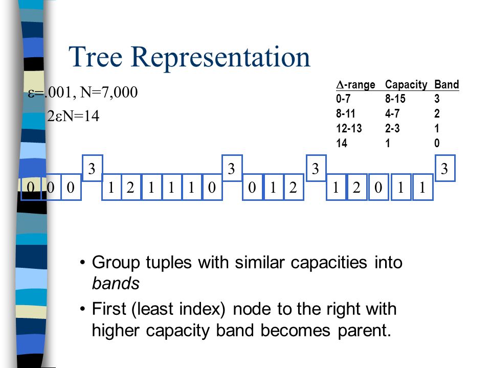
Tree Representation .001, N=7,000 2 N=14 -range CapacityBand 0-78-153 8-114-72 12-132-31 1410 000000111111112223333 Group tuples with similar capacities into bands First (least index) node to the right with higher capacity band becomes parent.
 node to the right with higher capacity band becomes parent.")
24
Tree Representation .001, N=7,000 2 N=14 -range CapacityBand 0-78-153 8-114-72 12-132-31 1410 Group tuples with similar capacities into bands First (least index) node to the right with higher capacity band becomes parent. 00000011111111222 3333
25
Tree Representation .001, N=7,000 2 N=14 -range CapacityBand 0-78-153 8-114-72 12-132-31 1410 Group tuples with similar capacities into bands First (least index) node to the right with higher capacity band becomes parent. 00000011111111 222 333 3

26
Tree Representation .001, N=7,000 2 N=14 -range CapacityBand 0-78-153 8-114-72 12-132-31 1410 Group tuples with similar capacities into bands First (least index) node to the right with higher capacity band becomes parent. 000000 1 111 1 1 11 2 22 333 3 R

27
Operation (compress) General strategy: delete tuples with small capacity and preserve tuples with large capacity. 1) Deletion cannot leave descendants unmerged --- it must delete entire subtrees 2) Deletion can only merge a tuple with small capacity into a tuple with similar or larger capacity. 3) Deletion cannot create an over-full tuple (i.e with g+ > floor(2 N))
 Deletion cannot leave descendants unmerged --- it must delete entire subtrees 2) Deletion can only merge a tuple with small capacity into a tuple with similar or larger capacity. 3) Deletion cannot create an over-full tuple (i.e with g+ > floor(2 N)).")
28
Analysis Theorem At any time n, the total number of tuples stored in S(n) is at most
 is at most")
29
Experimental Result Measurement: |S| Observed (vs. desired ) : max, avg, and for 16 representative quantiles Optimal max observed Compared 3 algorithms MRL Preallocated (1/3 number of stored observations as MRL) Adaptive: allocate a new quantile only when observed error is about to exceed desired
 : max, avg, and for 16 representative quantiles Optimal max observed Compared 3 algorithms MRL Preallocated (1/3 number of stored observations as MRL) Adaptive: allocate a new quantile only when observed error is about to exceed desired .")
30
Conclusion Better worst-case behavior than previous algorithms It does not require a priori knowledge of the parameter N

31
Any Question ?

Similar presentations


 A priority queue stores a collection of entries Each entry is a pair (key, value)>")


 Yossi Matias (Tel Aviv University) Viswanath Poosala.>")


 What is a B+ tree? Why B+ trees? Searching a B+ tree>")

 Rongfang Li Feb 2007.>")
. Can make sense because records may be much.>")
. Can make sense because records may be much.>")

