1. Tractable Higher Order Models in Computer Vision (Part II) Slides from Carsten Rother, Sebastian Nowozin, Pusohmeet Khli Microsoft Research Cambridge Presented by Xiaodan Liang

2. Part II Submodularity Move making algorithms Higher-order model : P n Potts model

3. Feature selection

4. Factoring distributions Problem inherently combinatorial!

5. Example: Greedy algorithm for feature selection

6. 6 s Key property: Diminishing returns Selection A = {} Selection B = {X 2,X 3 } Adding X 1 will help a lot! Adding X 1 doesn’t help much New feature X 1 B A s + + Large improvement Small improvement Submodularity: Y “Sick” X 1 “Fever” X 2 “Rash” X 3 “Male” Y “Sick” Theorem [Krause, Guestrin UAI ‘05] : Information gain F(A) in Naïve Bayes models is submodular!

7. 7 Why is submodularity useful? Theorem [Nemhauser et al ‘78] Greedy maximization algorithm returns A greedy : F(A greedy ) ¸ (1-1/e) max |A| k F(A) Greedy algorithm gives near-optimal solution! For info-gain: Guarantees best possible unless P = NP! [Krause, Guestrin UAI ’05] ~63%

8. 8 Submodularity in Machine Learning Many ML problems are submodular, i.e., for F submodular require: Minimization: A* = argmin F(A) – Structure learning (A* = argmin I(X A ; X V \ A )) – Clustering – MAP inference in Markov Random Fields –…–… Maximization: A* = argmax F(A) – Feature selection – Active learning – Ranking –…–…

9. Set functions

10. Submodular set functions Set function F on V is called submodular if Equivalent diminishing returns characterization: S B A S + + Large improvement Small improvement Submodularity: B A A [ B AÅBAÅB + + ¸

11. Submodularity and supermodularity

12. Example: Mutual information

13. 13 Closedness properties F 1,…,F m submodular functions on V and 1,…, m > 0 Then: F(A) =  i i F i (A) is submodular! Submodularity closed under nonnegative linear combinations! Extremely useful fact!! – F  (A) submodular )   P(  ) F  (A) submodular! – Multicriterion optimization: F 1,…,F m submodular, i ¸ 0 )  i i F i (A) submodular

14. 14 Submodularity and Concavity |A| g(|A|)

15. 15 Maximum of submodular functions Suppose F 1 (A) and F 2 (A) submodular. Is F(A) = max(F 1 (A),F 2 (A)) submodular? |A| F 2 (A) F 1 (A) F(A) = max(F 1 (A),F 2 (A)) max(F 1,F 2 ) not submodular in general!

16. 16 Minimum of submodular functions Well, maybe F(A) = min(F 1 (A),F 2 (A)) instead? F 1 (A)F 2 (A)F(A) ; 000 {a}100 {b}010 {a,b}111 F({b}) – F( ; )=0 F({a,b}) – F({a})=1 < But stay tuned min(F 1,F 2 ) not submodular in general!

17. 17 Duality For F submodular on V let G(A) = F(V) – F(V \ A) G is supermodular and called dual to F Details about properties in [Fujishige ’91] |A| F(A) |A| G(A)

18. 18 Submodularity and convexity

19. 19 The submodular polyhedron P F Example: V = {a,b} x({a}) · F({a}) x({b}) · F({b}) x({a,b}) · F({a,b}) PFPF x {a} x {b} 01 1 2 -2 AF(A) ; 0 {a} {b}2 {a,b}0

20. Lovasz extension

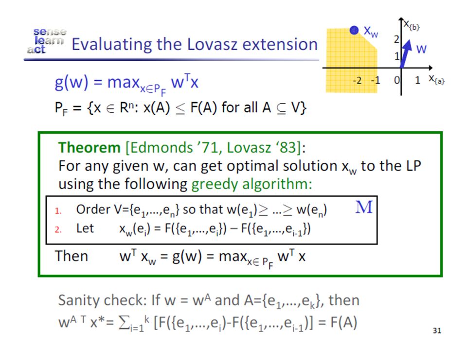
22. 22 w {a} w {b} 01 1 2 -2 Example: Lovasz extension g([0,1]) = [0,1] T [-2,2] = 2 = F({b}) g([1,1]) = [1,1] T [-1,1] = 0 = F({a,b}) {}{a} {b}{a,b} [-1,1] [-2,2] g(w) = max {w T x: x 2 P F } w=[0,1] want g(w) Greedy ordering: e 1 = b, e 2 = a  w(e 1 )=1 > w(e 2 )=0 x w (e 1 )=F({b})-F( ; )=2 x w (e 2 )=F({b,a})-F({b})=-2  x w =[-2,2] AF(A) ; 0 {a} {b}2 {a,b}0

23. 23 Why is this useful? Theorem [Lovasz ’83]: g(w) attains its minimum in [0,1] n at a corner! If we can minimize g on [0,1] n, can minimize F… (at corners, g and F take same values) F(A) submodular g(w) convex (and efficient to evaluate) Does the converse also hold? No, consider g(w 1,w 2,w 3 ) = max(w 1,w 2 +w 3 ) {a}{b}{c} F({a,b})-F({a})=0 < F({a,b,c})-F({a,c})=1

24. Minimizing a submodular function Ellipsoid algorithm Interior Points algorithm

25. Example: Image denoising

26. 26 Example: Image denoising X1X1 X4X4 X7X7 X2X2 X5X5 X8X8 X3X3 X6X6 X9X9 Y1Y1 Y4Y4 Y7Y7 Y2Y2 Y5Y5 Y8Y8 Y3Y3 Y6Y6 Y9Y9 P(x 1,…,x n,y 1,…,y n ) =  i,j  i,j (y i,y j )  i  i (x i,y i ) Want argmax y P(y | x) =argmax y log P(x,y) =argmin y  i,j E i,j (y i,y j )+  i E i (y i ) When is this MAP inference efficiently solvable (in high treewidth graphical models)? E i,j (y i,y j ) = -log  i,j (y i,y j ) Pairwise Markov Random Field X i : noisy pixels Y i : “true” pixels

27. MAP inference in Markov Random Fields [Kolmogorov et al, PAMI ’04, see also: Hammer, Ops Res ‘65]

28. 28 Constrained minimization

29. Part II Submodularity Move making algorithms Higher-order model : P n Potts model

30. Multi-Label problems

31. Move making expansions move and swap move for this problem

32. Metric and Semi metric Potential functions

33. if the pairwise potential functions define a metric then the energy function in equation (8) can be approximately minimized using alpha expansions. if pairwise potential functions defines a semi- metric, it can be minimized using alpha beta- swaps.

34. Move Energy Each move: A transformation function: The energy of a move t: The optimal move: Submodular set functions play an important role in energy minimization as they can be minimized in polynomial time

35. The swap move algorithm

36. The expansion move algorithm

37. Higher order potential The class of higher order clique potentials for which the expansion and swap moves can be computed in polynomial time The clique potential take the form:

38. Question you should be asking: Show that move energy is submodular for all x c Can my higher order potential be solved using α-expansions?

39. Form of the Higher Order Potentials Moves for Higher Order Potentials Clique Inconsistency function: Pairwise potential: xixi xjxj xkxk xmxm xlxl c Sum Form Max Form

40. Theoretical Results: Swap Move energy is always submodular if non-decreasing concave. proofs

41. Condition for Swap move Concave Function:

42. Prove all projections on two variables of any alpha beta-swap move energy are submodular. The cost of any configuration

43. substitute Constraints 1: Lema 1: Constraints2:

44. Condition for alpha expansion Metric:

45. Form of the Higher Order Potentials Moves for Higher Order Potentials Clique Inconsistency function: Pairwise potential: xixi xjxj xkxk xmxm xlxl c Sum Form Max Form

46. Part II Submodularity Move making algorithms Higher-order model : P n Potts model

47. Image Segmentation E(X) = ∑ c i x i + ∑ d ij |x i -x j | ii,j E: {0,1} n → R 0 → fg, 1 → bg n = number of pixels [Boykov and Jolly ‘ 01] [Blake et al. ‘04] [Rother et al.`04] Image Unary Cost Segmentation

48. P n Potts Potentials Patch Dictionary (Tree) C max  0 { 0 if x i = 0, i p C max otherwise h(X p ) = p [slide credits: Kohli]

49. P n Potts Potentials E(X) = ∑ c i x i + ∑ d ij |x i -x j | + ∑ h p (X p ) ii,j p p { 0 if x i = 0, i p C max otherwise h(X p ) = E: {0,1} n → R 0 → fg, 1 → bg n = number of pixels [slide credits: Kohli]

50. Theoretical Results: Expansion Move energy is always submodular if increasing linear See paper for proofs

51. P N Potts Model c

52. c Cost : 

53. P N Potts Model c Cost :  max

54. Optimal moves for P N Potts Computing the optimal swap move c Label 3 Label 4 Case 1 Not all variables assigned label 1 or 2 Move Energy is independent of t c and can be ignored. Label 1  Label 2 

55. Optimal moves for P N Potts Computing the optimal swap move c Label 1  Label 2  Label 3 Label 4 Case 2 All variables assigned label 1 or 2

56. Optimal moves for P N Potts Computing the optimal swap move c Label 3 Label 4 Case 2 All variables assigned label 1 or 2 Can be minimized by solving a st- mincut problem Label 1  Label 2 

57. Solving the Move Energy Add a constant This transformation does not effect the solution add a constant K to all possible values of the clique potential without changing the optimal move

58. Solving the Move Energy Computing the optimal swap move Source Sink v1v1 v2v2 vnvn MsMs MtMt t i = 0 v i  Source Set t j = 1 v j  Sink Set

59. Solving the Move Energy Computing the optimal swap move Case 1: all x i =  (v i  Source ) Cost: Source Sink v1v1 v2v2 vnvn MsMs MtMt

60. Solving the Move Energy Computing the optimal swap move v1v1 v2v2 vnvn MsMs MtMt Cost: Source Sink Case 2: all x i =  (v i  Sink )

61. Solving the Move Energy Computing the optimal swap move Cost: v1v1 v2v2 vnvn MsMs MtMt Source Sink Case 3: all x i =  (v i  Source, Sink ) Recall that the cost of an st-mincut is the sum of weights of the edges included in the stmincut which go from the source set to the sink set.

62. Optimal moves for P N Potts The expansion move energy Similar graph construction.

63. Experimental Results Texture Segmentation Unary (Colour) Pairwise (Smoothness) Higher Order (Texture) Original PairwiseHigher order

64. Experimental Results OriginalSwap (3.2 sec) Expansion (2.5 sec) PairwiseHigher Order Swap (4.2 sec) Expansion (3.0 sec)

65. Experimental Results Original PairwiseHigher Order Swap (4.7 sec) Expansion (3.7sec) Swap (5.0 sec) Expansion (4.4 sec)

66. More Higher-order models