1. Yan Y. Kagan
Dept. Earth and Space Sciences, UCLA, Los Angeles, CA ,
WHY DOES THEORETICAL PHYSICS FAIL TO EXPLAIN AND PREDICT EARTHQUAKE OCCURRENCE?

2. Several reasons can be proposed:
1. Multidimensional character of seismicity: earthquake time, space, size, and focal mechanism need to be modeled. The latter is a symmetric second-rank tensor of special kind.
2. Intrinsic randomness of the earthquake occurrence, the need to apply the theory of stochastic point processes and appropriate complex statistical techniques.

3. 3. Scale-invariant or fractal properties of earthquake process; the theory of random stable or heavy-tailed variables is significantly more difficult than that of Gaussian variables and is only being currently developed. The earthquake process theory should be renormalizable.
4. Statistical distributions of earthquake size, earthquake temporal interaction, their spatial patterns and focal mechanisms are largely universal with the values of major parameters similar for earthquakes in various tectonic zones. The universality of these distributions gives us some hope in creating foundations for earthquake process theory.

4. 5. The quality of current earthquake data statistical analysis is low; little or no study of random and systematic errors is usually performed, thus most of the published statistical results are artifacts.
6. Earthquake process does not operate as an isolated system. Scale-invariance of the process means that the largest inhomogeneity of earthquake fault system (defect) is comparable in size with the region
extent, same for the next largest defect, etc. Thus, in any seismic region we cannot separate the largest fault or fault system and treat the remainder as medium with uniform properties.

5. 7. During earthquake rupture propagation focal mechanisms sometimes undergo large 3-D rotations. This necessitates applying non-commutative
algebra (e.g., quaternions and gauge theory) to model earthquake occurrence. Almost all field theories currently employed in physics are based on complex numbers, i.e., use commutative algebra.
8. These phenomenological and theoretical difficulties are not limited to earthquakes; any fracture of brittle materials, tensile or shear, would encounter similar problems.

6. Lecture Outline 1. Deficiencies of present physical models.
2. Earthquake occurrence phenomenology: fractal distributions of size, time, space, and focal mechanisms.
3. Fractal model of earthquake process: random stress interactions.
4. Statistical forecasting of earthquakes and its testing.

7. Two major unsolved problems of modern science
1. Turbulent flow of fluids (Navier-Stocks equations).
2. Brittle fracture of solids.
Plastic deformation of materials is an intermediate case: it behaves as a solid for short-term interaction and as a liquid for long-term interaction.
Kagan, Y. Y., Seismicity: Turbulence of solids, Nonlinear Science Today, 2, 1-13.

8. Navier-Stokes Equation
“Waves follow our boat as we meander across the lake, and turbulent air currents follow our flight in a modern jet. Mathematicians and physicists believe that an explanation for and the prediction of both the breeze and the turbulence can be found through an understanding of solutions to the Navier-Stokes equations. Although these equations were written down in the 19-th Century, our understanding of them remains minimal. The challenge is to make substantial progress toward a mathematical theory which will unlock the secrets hidden in the Navier-Stokes equations.”
(Clay Institute -- prize $1 M).

9. Akiva Yaglom (2001, p. 4) commented that the turbulence status is different from many other complex problems that 20-th century physics solved or have been trying to solve: "However, turbulence theory deals with the most ordinary and simple realities of the everyday life such as, e.g., the jet of water spurting from the kitchen tap."
Nevertheless, the turbulence problem is not among the ten millennium problems in physics presented by University of Michigan Ann Arbor, see
or 11 problems by the National Research Council's Board on Physics and Astronomy (Haseltine, Discover, 2002).

10. Horace Lamb on Turbulence (1932)
“I am an old man now, and when I die and go to Heaven there are two matters on which I hope for enlightenment. One is quantum electrodynamics, and the other is the turbulent motion of fluids. And about the former I am really rather optimistic.”
Goldstein, S., Fluid mechanics in the first half of this century, Annual Rev. Fluid Mech., 1, p. 23.
This story is apocryphally repeated with Einstein, von Neumann, Heisenberg, Feynman, and others.

11. Brittle Fracture of Solids
Similarly, brittle fracture of solids is commonly encountered in everyday life, and still there is no real theory explaining its properties or predicting the outcome of the simplest occurrences, like breaking a glass. It is certainly a much more difficult scientific problem than turbulence, and while the turbulence attracted first-class mathematicians and physicists, no such interest has been shown in mathematical theory of fracture and large-scale deformation of solids.
Kagan, Y. Y., Seismicity: Turbulence of solids, Nonlinear Science Today, 2, 1-13.

12. Columbia Accident Investigation Board, Report, Volume I, 2003,

13. O'Brien, J. F., and Hodgins, J. K. 1999.
Graphical modeling and animation of brittle fracture, Proceedings of Assoc. Computing Machinery (ACM) SIGGRAPH 99,

14. Seismicity Model
This picture represent a paradigm of the current earthquake physics. Originally, when Burridge and Knopoff proposed this model in 1967, this was the first mathematical treatment of earthquake rupture, a very important development.

15. Seismicity model
Since then perhaps hundreds papers have been published using this model or its variants. We show below that presently much more complicated mathematical tools are needed to represent brittle shear earthquake fracture.

16. The model must be modernized. Why?
1. It is a closed, isolated system, whereas tectonic earthquakes occur in an open environment. This model justifies spurious quasi-periodicity, seismic gaps, and seismic cycle models.
No rigorous observational evidence exists for the presence of these features (Rong et al., JGR, 2003).

17. The model must be modernized. Why?
2. Earthquake fault in the model is a well-defined geometrical object -- a planar surface with dimension 2. In nature only earthquake fault system exists as a fractal set. This set is not a surface, its dimension is about 2.2.

18. Kagan, Y. Y., Stochastic model of earthquake fault geometry, Geophys. J. R. astr. Soc., 71,

19. The model must be modernized. Why?
3. Several distinct scales are present in the diagram: inhomogeneity of planar surface, plates size. Earthquakes are scale-invariant. Geometry and mechanical properties of the earthquake fault zone are the result of self-organization. They are fractal.

20. The model must be modernized. Why?
4. Incompatibility problem is circumvented because of flat plate boundaries. Real earthquake faults always contain triple junctions; further deformation is impossible without creating new fractures and rotational defects (disclinations).

21. Example of geometric incompatibility near fault junction
Example of geometric incompatibility near fault junction. Corners A and C are either converging and would overlap or are diverging; this indicates that the movement cannot be realized without the change of the fault geometry (Gabrielov, A., Keilis-Borok, V., and Jackson, D. D., Geometric incompatibility in a fault system, P. Natl. Acad. Sci. USA, 93, ).

22. The model must be modernized. Why?
5. Because of planar boundaries, stress concentrations are practically absent after a major earthquake. Hence few or no aftershocks.
Kagan and Knopoff (JGR,1981); Kagan (GJRAS, 1982) proposed a new model of earthquake occurrence, based on fractal geometry and 3-D rotation of mechanisms.

23. The model must be modernized. Why?
6. All earthquakes in the model have the same focal mechanism. Variations of mechanisms that are obvious even during a cursory inspection of focal mechanism maps are not taken into account.
Kagan (2000). Temporal correlations of earthquake focal mechanisms, Geophys. J. Int., 143,

24. Characteristic Earthquakes, Seismic Gaps, Quasi-periodicity
Schwartz and Coppersmith (1984) proposed the characteristic model. McCann et al. (1979) and Nishenko (1991) formulated testable hypothesis -- about 100 zones in circum-Pacific belt. Kagan & Jackson (JGR, 1991, 1995), and Rong et al. (JGR, 2003) tested these predictions and found that earthquakes after 1979 or 1989, respectively, do not support the model.

25. McCann et al. (1979) The map of seismic gap zones -- compare Sumatra 2004 rupture.
Kagan & Jackson (1991) tested the map – the result is negative.

26. Characteristic Earthquakes, Seismic gaps, Quasi-periodicity
Bakun & Lindh (Science, 1985) -- Parkfield prediction, 95% probability of M6 event in No earthquake occurred. In 2004 M6 event in the Parkfield area. Only few of the predicted features were observed. Bakun et al. (Nature, 2005) review the experiment results -- no new prediction is issued. See Jackson & Kagan (2006) ~ykagan/parkf2004_index.html.

27. Characteristic Earthquakes, Seismic Gaps, Quasi-periodicity
Chris Scholz in the 1999 Nature Debate:
In their [Kagan & Jackson] more recent study, they found, in contrast, less events than predicted by Nishenko [1991]. But here the failure was in a different part of the physics: the assumptions of recurrence times made by Nishenko. These recurrence times are based on very little data, no theory, and are unquestionably suspect.

28. Characteristic Earthquakes, Seismic Gaps, Quasi-periodicity
Bakun et al., Nature, 2005:
(The characteristic earthquake model can also
be tested using global data sets. Kagan and Jackson [1995] concluded that too few of Nishenko’s [1991] predicted gap-filling circum-Pacific earthquakes occurred in the first 5 yr.)

29. Characteristic Earthquakes, Seismic Gaps, Quasi-periodicity
Despite the failure of these predictions, this model was employed in San Francisco Bay area (Working Group, 2003) -- "there is a 0.62 [ ] probability of a major, damaging [M > 6.7] earthquake striking the greater San Francisco Bay Region over the next 30 years ( )."

30. Characteristic Earthquakes, Seismic Gaps, Quasi-periodicity
Stark and Freedman (2003) argue that the probabilities defined in such a prediction are meaningless because they cannot be validated. They suggest that the reader "should largely ignore the USGS probability forecast."
See more detail in Jackson & Kagan (2006)

31. Characteristic Earthquakes, Seismic Gaps, Quasi-periodicity
Thomas Kuhn (1965) questioned how one can distinguish scientific and non-scientific predictions. As an example, he used astronomy versus astrology -- both issue predictions that sometimes fail. However, astronomers learn from these mistakes, modify and update their models, whereas astrologers do not.

32. Current Physical Models of Seismicity
Dieterich, JGR, 1994; Rice and Ben-Zion, Proc. Nat. Acad., 1996; Langer et al., Proc. Nat. Acad., 1996, see also review by Kanamori and Brodsky, Rep. Prog. Phys., their major paradigm: two blocks separated by a planar boundary.

33. Current Physical Models of Seismicity
These models describe only one boundary between blocks; they do not account for a complex interaction of other block boundaries and, in particular, its triple junctions. Seismic maps convincingly demonstrate that earthquakes occur mostly at boundaries of relatively rigid blocks. This is the major idea of the plate tectonics. However, if blocks are rigid, stress concentrations at other block boundaries and blocks’ triple junctions should influence the earthquake pattern at any particular boundary.

34. Current Physical Models of Seismicity
No rigorous testing of these models is performed. At the present time, numerical earthquake models have shown no predictive capability exceeding or comparable to the empirical prediction based on earthquake statistics. Examples are selectively chosen data. These models have a large number of adjustable parameters, both obvious and hidden, to simulate seismic activity.

35. Current seismicity physical models
Enrico Fermi: “I remember my friend Johnny von Neumann used to say, with four parameters I can fit an elephant, and with five I can make him wiggle his trunk.”
Dyson, Nature, 427(6972), 297.

36. Current Physical Models of Seismicity
The models 'successfully' claim as their consequence some artifacts or non-existent phenomena, such as characteristic earthquakes or non-zero value for the c-coefficient in Omori's law.
They are less successful in solving pseudo-problems of their own creation, such as heat flow paradox or strength of earthquake faults.

37. Earthquake Phenomenology
Modern earthquake catalogs include origin time, hypocenter location, and second-rank seismic moment tensor for each earthquake. The tensor is symmetric, traceless, with zero determinant: hence it has only four degrees of freedom -- one for the norm of the tensor and three for the 3-D orientation of the earthquake focal mechanism. An earthquake occurrence is considered to be a stochastic, tensor-valued, multidimensional, point process.

38. Southern California earthquake epicenters: black -- wave-correlation method; color – standard (first arrival) method. Accuracy of the first method is tens of m, of the second – about 1 km.

39. Statistical Studies of Earthquake Catalogs: Time, Size, Space
Catalogs are a major source of information on earthquake occurrence.
Since late 19-th century certain statistical features were established: Omori (1894) studied temporal distribution; Gutenberg & Richter (1941; 1944) -- size distribution.
Quantitative investigations of spatial patterns started late (Kagan & Knopoff, 1980).

40. Southern California earthquakes 1800-2005
Blue -- focal
mechanisms
determined.
Orange --
Mechanisms
estimated
through
interpolation

41. Statistical Studies of Earthquake Catalogs: moment tensor
Kostrov (1974) proposed that earthquake can be described by a second-rank tensor. Gilbert & Dziewonski (1975) first obtained the tensor solution from seismograms.
However, statistical investigations even now remain largely restricted to time-size-space regularities.
Why? Statistical tensor analysis requires entry to truly modern mathematics.

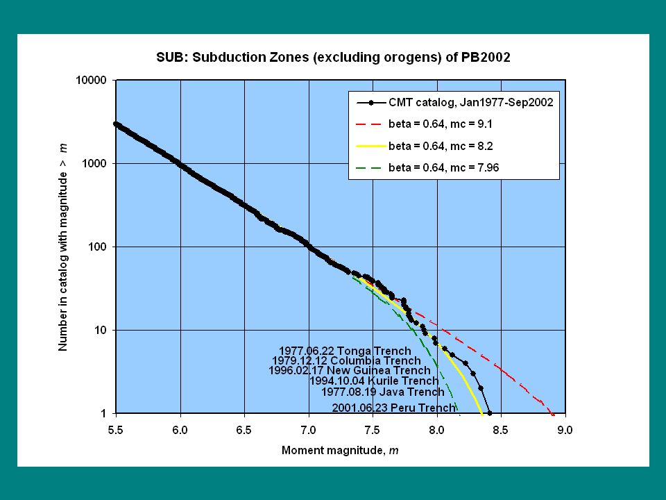
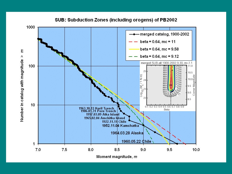
43. Observational Results
Earthquake process exhibits scale-invariant, fractal properties:
(1) Earthquake size distribution is a power-law (Gutenberg-Richter) with an exponential tail. The power-law exponent has a universal value for all earthquakes. The maximum (corner) magnitude values are determined for major tectonic provinces.
(2) The temporal fractal pattern is power-law decay of the rate of the aftershock and foreshock occurrence (Omori's law). Power-law time pattern can be extended to small time intervals explaining the complex structure of the earthquake rupture process.
(3) Spatial distribution of earthquakes is fractal; the correlation dimension of earthquake hypocenters is about 2.2 for shallow earthquakes.
(4) Disorientation of earthquake focal mechanisms is approximated by the rotational 3-D Cauchy distribution.

44. Using the Harvard CMT catalog of 15,015 shallow events:

47. Review of results on spectral slope, b:
Although there are variations, none is significant with 95%-confidence.
Kagan’s [1999] hypothesis of uniform b still stands.

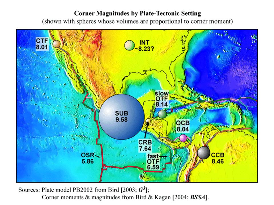
49. IMPLICATIONS:
Now that we know the coupled thickness of the seismogenic lithosphere in each tectonic setting, we can convert surface velocity gradients to seismic moment rates.
Now that we know the frequency/magnitude distribution in each tectonic setting, we can convert seismic moment rates to earthquake rate densities at any desired magnitude.
Long-term-average
(Poissonian)
seismicity maps
Kinematic
Model
Moment
Rates

50. Relation Between Moment Sums and Tectonic Deformation
From the beginning of the plate tectonics hypothesis it was assumed that earthquakes are due to plate boundaries deformation.
Calculations for global tectonics and large seismic regions justified such approach.
However, application of this assumption to smaller regions has usually been inconclusive due to high variability of seismic moment sums.

51. Holt, W. E., Chamot-Rooke, N., Le Pichon, X., Haines, A. J.,
Shen-Tu, B., and Ren, J., Velocity field in Asia inferred from Quaternary fault slip rates and Global Positioning System observations, J. Geophys. Res., 105, 19,185-19,209.

52. Zaliapin, I. V. , Y. Y. Kagan, and F. Schoenberg, 2005
Zaliapin, I. V., Y. Y. Kagan, and F. Schoenberg, Approximating the distribution of Pareto sums, Pure Appl. Geoph. (PAGEOPH), 162(6-7),

54. Non-linear increase of sums of heavy-tailed distributions may explain accelerated moment or Benioff strain release (Bufe & Varnes, 1993, and many others) .

55. Sumatra M 9.1 earthquake

56. Cross -- Harvard catalog; Blue stars -- PDE catalog;
Green dots -- CalTech catalog.

57. Kagan, Y. Y., and H. Houston, 2005. Relation between mainshock rupture process
and Omori's law for aftershock moment release rate, Geophys. J. Int., 163(3),

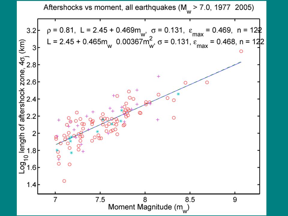
58. Earthquake Scaling: M ~ L3
It is commonly believed that the earthquake focal size scaling (i.e., dependence of the size on seismic moment) is different for events of various focal mechanisms.
In particular, strike-slip earthquakes which occur on vertical faults are considered to have two power-law dependencies: break occurring around km (corresponding to M6 event).
Long debate between Scholz and Romanowicz.

59. Aftershock map for 1997/12/5 Kamchatka earthquake
(M = 5.32*10^20 Nm, m= 7.82).
Stars -- aftershock epicenters, cross -- average aftershock
position, circle -- centroid vertical projection
onto the Earth surface, diamond -- NEIC mainshock epicenter.
Two-dimensional Gaussian approximation of aftershock
distribution is shown.

61. Earthquakes :
Mw (CMT), aftershocks (PDE)

62. Earthquakes

63. Spatial Distribution of Earthquakes
We measure distances between pairs, triplets, and quadruplets of events.
The distribution of distances, triangle areas, and tetrahedron volumes turns out to be fractal, i.e., power-law.
The power-law exponent depends on catalog length, location errors, depth distribution of earthquakes. All this makes statistical analysis very difficult.

64. Spatial Moments: Two- Three- and Four-point functions;
Distribution of distances (D), surface areas (S), and volumes (V) of point simplexes is studied. The probabilities are approximately 1/D, 1/S, and 1/V.

65. Distribution of distances between hypocenters N(R,t) for the Hauksson & Shearer (2005) catalog, using only earthquake pairs with inter-event times in the range
[t, 1.25t]. Time interval t increases between 1.4 minutes (blue curve) to 2500 days (red curve). See Helmstetter, Kagan & Jackson (JGR, 2005).

66. New ms -- http://scec.ess.ucla.edu/~ykagan/p2rev_index.html

67. Earthquake Focal Mechanism
Double-couple tensor M = M diag [1, -1, 0] has 4 degrees of freedom, since its 1st and 3rd invariants are zero. The normalized tensor corresponds to a normalized quaternion q = (0, 0, 0, 1). Arbitrary double-couple source is obtained by multiplying the initial quaternion by a quaternion representing a 3-D rotation (see Kagan, GJI, 163(3), , 2005).

68. Kagan, Y. Y., 1992.
Correlations of earthquake focal mechanisms,
Geophys. J. Int., 110,
Upper picture -- distance 0-50 km.
Lower picture -- distance km.
Upper solid line -- Cauchy distribution;
Dashed line - random rotation.

69. Kagan, Y. Y., Temporal correlations of earthquake focal mechanisms, Geophys. J. Int., 143,

70. Stress and Earthquakes
Stress due to past earthquakes can be calculated with reasonable accuracy.
Evaluation of tectonic stress is more difficult, especially for smaller scales.
Incremental stress is found to be distributed according to Cauchy distribution, the behavior predicted by Zolotarev (1983).
Rotation of focal mechanisms is governed by Cauchy distribution.

71. Focal mechanisms of earthquakes for in the southern California area and major surface faults. Lower hemisphere diagrams of focal spheres are shown; the diagrams can be thought of as 3-D rotations of the mechanism. All events with magnitude m >= 6.5 are replaced by extended sources, containing several smaller rectangular dislocation patches matching total earthquake moment.
Kagan, Jackson, and Liu, Stress and earthquakes in southern California, ,
J. Geophys. Res., 110(5), B05S14

72. Branching Model for Dislocations (Kagan and Knopoff, JGR,1981; Kagan, GJRAS, 1982)
Predates use of self-exciting, ETAS models which also have branching structure.
A more complex model, exists on a more fundamental level.
Continuum-state critical branching random walk in T x R3 x SO(3).
Many unresolved claims, mathematical issues: is the synthetic earthquake set scale-invariant?

73. Critical branching process --genealogical tree of simulations

74. (a) Pareto distribution
of time intervals time^(1-u)
(b) Rotation of focal mechanisms follows a Cauchy distribution

75. Simulated source-time functions and seismograms for shallow earthquake sources. The upper trace is a synthetic source-time function. The middle plot is a theoretical seismogram, and the lower trace is a convolution of the derivative of source-time function with the theoretical seismogram.
Kagan, Y. Y., and Knopoff, L., Stochastic synthesis of earthquake catalogs, J. Geophys. Res., 86,

76. Kagan, Y. Y., and Knopoff, L., Random stress and earthquake statistics: Time dependence, Geophys. J. R. astr. Soc., 88,

77. Snapshots of a fault propagation, simulated fault
Snapshots of a fault propagation, simulated fault. Integers in the frames # indicate the numbers of elementary events to which these frames correspond. Ten frames on the left show the development of an earthquake sequence in the whole area. The frames on the right are magnifications of the parts enclosed in rectangles.

78. Non-commutability of 3-D rotations presents a major difficulty in creating probabilistic theory of earthquake rupture propagation

79. Hamilton's letter to his son
Every morning in the early part of the above-cited month [October 1843], on my coming down to breakfast, your (then) little brother William Edwin, and yourself, used to ask me: "Well, Papa, can you multiply triplets?" Whereto I was always obliged to reply, with a sad shake of the head: `No, I can only add and subtract them".

80. Brougham Bridge, Dublin
Here as he walked by on the 16th of October 1843 Sir William Rowan Hamilton in a flash of genius discovered the fundamental formula for quaternion multiplication & cut it on a stone of this bridge.

81. Libicki, E. , and Y. Ben-Zion, 2005
Libicki, E., and Y. Ben-Zion, Stochastic Branching Models of Fault Surfaces and Estimated Fractal Dimension,
Pure Appl. Geophys., 162(6-7),

82. Simulation Results:
A model of random defect interaction in a critical stress environment explains most of the available empirical statistical results.
Omori's law is a consequence of a Brownian motion-like behavior of random stress due to defect dynamics.
The evolution and self-organization of defects in the rock medium are responsible for the fractal spatial patterns of earthquake faults.

83. Simulation Results:
The Cauchy and other symmetric stable distributions govern the stress caused by these defects.
Random rotation of focal mechanisms is controlled by the rotational Cauchy and other stable distributions.
Orientation of these dislocations is defined by a normalized quaternion (3 DF), but they determine the random stress (6 DF).

84. Probabilistic vs. alarm forecasts
A modern scientific earthquake forecast should be quantitatively probabilistic. In 1654 Pierre de Fermat and Blaise Pascal exchanged letters in which they founded the quantitative probability theory. Now more than 350 years later, any earthquake forecast without direct use of probability has a medieval flavor. This is perhaps the reason the general public and media are so attracted to yes/no forecasts.

85. Earthquake Probability Forecasting
The fractal dimension of earthquake process is lower than the embedding dimension:
Time – 0.5 in 1D
Space – 2.2 in 3D
Focal mechanisms – Cauchy distribution
This allows us to forecast probability of earthquake occurrence – specify regions of high probability, use temporal clustering for evaluating possibility of new event and predict its focal mechanism.

86. (a) Earthquake
catalog data
(b) Point process branching along magnitude axis, introduced by Kagan (1973a;b)
(c) Point process branching along time axis (Hawkes, 1971; Kagan & Knopoff, 1987; Ogata, 1988)

87. Here we
demonstrate
forecast
effectiveness:
displayed
earthquakes
occurred after
smoothed
seismicity forecast
was calculated.

88. Time history of long-term and hybrid (short-term plus 0.8 *
long-term) forecast for a point at latitude N., E. northwest of Honshu Island, Japan. Blue line is the long-term forecast; red line is the hybrid forecast.

89. Short-term forecast uses Omori's law to
extrapolate present
seismicity.
Red spot east of
Honshu Island is
the consequence of the M7 2005/11/14
earthquake

90. Forecast Efficiency Evaluation
We simulate synthetic catalogs using smoothed seismicity map.
Likelihood function for simulated catalogs and for real earthquakes in the time period of forecast is computed.
If the `real earthquakes’ likelihood value is within 2.5—97.5% of synthetic distribution, the forecast is considered successful.
Kagan, Y. Y., and D. D. Jackson, Probabilistic forecasting of earthquakes, (Leon Knopoff's Festschrift), Geophys. J. Int., 143,

92. Kossobokov, Testing earthquake prediction methods: ``The West Pacific short-term forecast of earthquakes with magnitude MwHRV \ge 5.8", Tectonophysics, 413(1-2),
See also Kagan & Jackson, pp

93. Earthquake prediction and its optimization,
Molchan, G. M., and Y. Y. Kagan, 1992.
Earthquake prediction and its optimization,
J. Geophys. Res., 97,

94. Kagan, Y. Y., and Knopoff, L., A stochastic model of earthquake occurrence, Proc. 8-th Int. Conf. Earthq. Eng., 1,

95. Conclusions
The major theoretical challenge in describing earthquake occurrence is to create scale-invariant models of stochastic processes, and to describe geometrical/topological and group-theoretical properties of stochastic fractal tensor-valued fields (stress/strain, earthquake focal mechanisms).
It needs to be done in order to connect phenomenological statistical results and attempts at earthquake occurrence modeling with a non-linear theory appropriate for large deformations.
The statistical results can also be used to evaluate seismic hazard and to reprocess earthquake catalog data in order to decrease their uncertainties.

96. End Thank you

97. Earthquake Probability Forecasting
The fractal dimension of earthquake process is lower than the embedding dimension:
Space – 2.2 in 3D
Time – 0.5 in 1D
This allows us to forecast probability of earthquake occurrence – specify regions of high probability and use temporal clustering to evaluate the possibility of a new event.