1. ERCOT UFE Analysis UFE Task Force February 21, 2005

2. Introduction UFE Cost and Scenario Analysis UFE by Weather Zone UFE Allocation Calculation of Distribution Losses

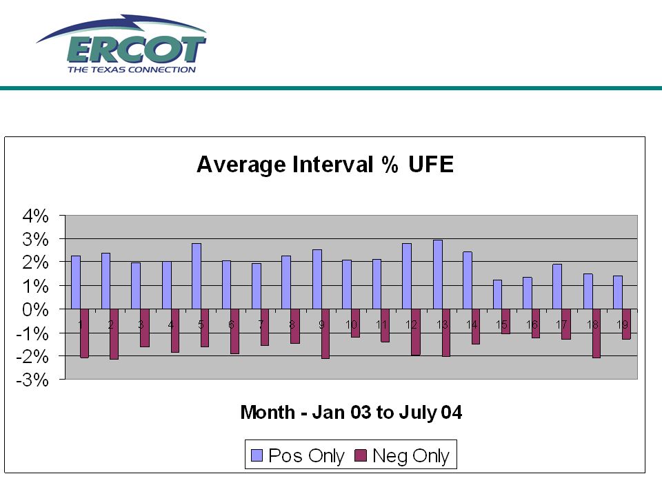
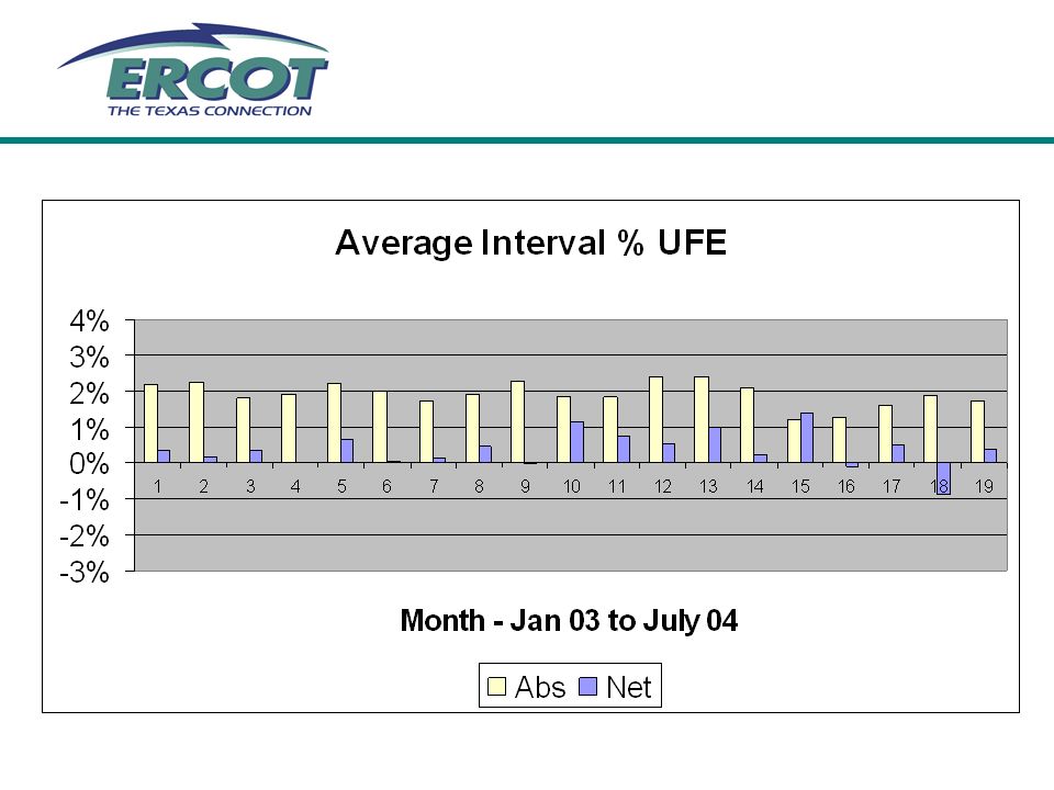
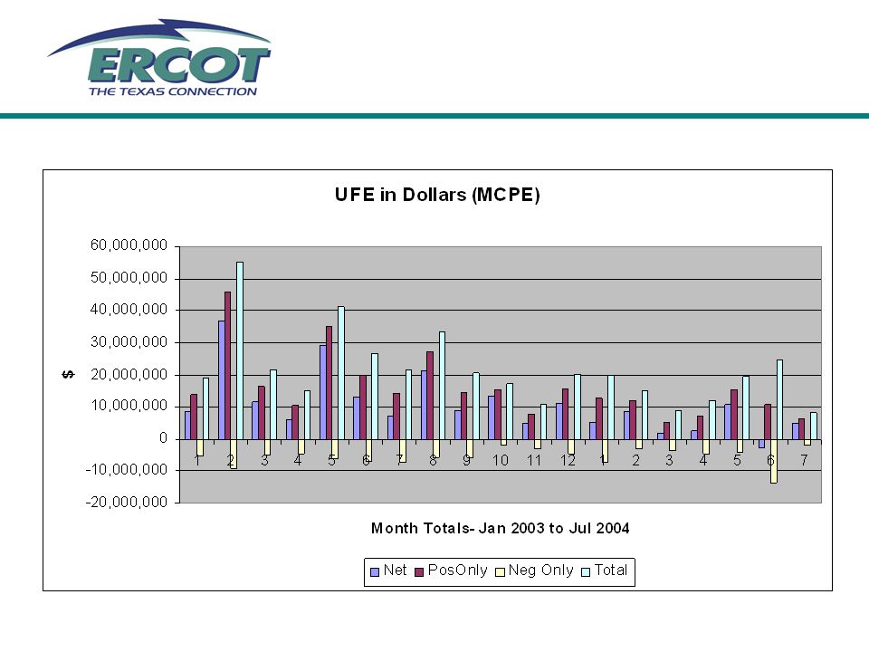
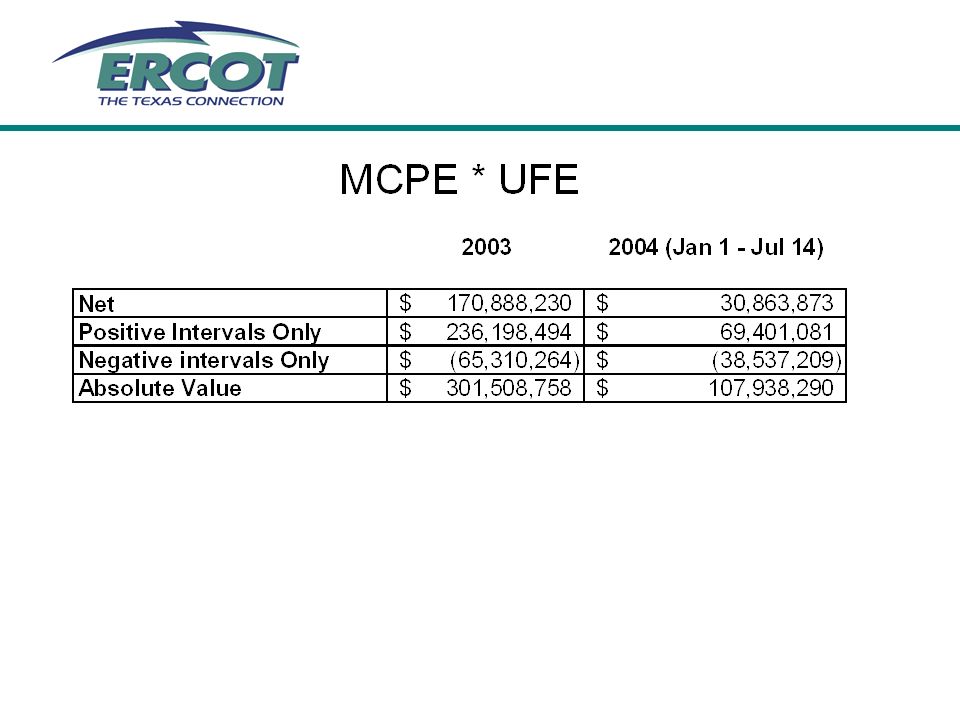
3. UFE Cost Associating dollar values (not costs) with UFE … can we get some sense of whether/how much investment to make improvements is justified? MCPE × UFE is a reasonable approximation How to handle intervals with negative MCPE and/or negative UFE? (note: negative MCPE is rare ~ 0.5% of intervals in 2003) Consider some slides from ERCOT’s presentation at September 14 UFE Workshop

8. UFE Scenario Analysis Consider some simplified scenarios to aid in the understanding of the implications of negative UFE and disproportionate UFE

9. Scenario 1 – Negative UFE QSE 1 load = QSE 2 load QSE 1 over-estimated by 10%, QSE 2 under-estimated by 5% UFE is -2.5% Following UFE adjustment QSE 1 is over-estimated by 7.32% QSE 2 is under-estimated by 7.32% UFE understates actual error

10. Scenario 1 – Positive UFE QSE 1 load = QSE 2 load QSE 1 over-estimated by 5%, QSE 2 under-estimated by 10% UFE is +2.5% Following UFE adjustment QSE 1 is over-estimated by 7.69% QSE 2 is under-estimated by 7.69% UFE understates actual error

11. Scenario 2 – Negative UFE QSE 1 load = QSE 2 load QSE 1 over-estimated by 5%, QSE 2 is correct UFE is -2.5% Following UFE adjustment QSE 1 is over-estimated by 2.44% QSE 2 is under-estimated by 2.44% UFE overstates actual error

12. Scenario 2 – Positive UFE QSE 1 load = QSE 2 load QSE 1 under-estimated by 5%, QSE 2 is correct UFE is +2.5% Following UFE adjustment QSE 1 is under-estimated by 2.56% QSE 2 is over-estimated by 2.56% UFE understates actual error

13. Scenario 3 – Negative UFE QSE 1 load = QSE 2 load QSE 1 over-estimated by 4%, QSE 2 over-estimated by 1% UFE is -2.5% Following UFE adjustment QSE 1 is over-estimated by 1.46% QSE 2 is under-estimated by 1.46% UFE overstates actual error

14. Scenario 3 – Positive UFE QSE 1 load = QSE 2 load QSE 1 under-estimated by 4%, QSE 2 under-estimated by 1% UFE is +2.5% Following UFE adjustment QSE 1 is under-estimated by 1.54% QSE 2 is over-estimated by 1.54% UFE overstates actual error

15. Scenario 4 – Negative UFE QSE 1 load = QSE 2 load QSE 1 over-estimated by 2.5%, QSE 2 over-estimated by 2.5% UFE is -2.5% Following UFE adjustment QSE 1 and QSE 2 are correctly estimated UFE overstates actual error

16. Scenario 5 – Negative UFE – QSEs with Different Load Ratio Shares QSE 1 load > QSE 2 load QSE 1 over-estimated by 4%, QSE 2 over-estimated by 1% UFE is -2.88% Following UFE adjustment QSE 1 is over-estimated by 1.09% QSE 2 is under-estimated by 1.82% UFE overstates actual error

17. Scenario 5 – Positive UFE – QSEs with Different Load Ratio Shares QSE 1 load > QSE 2 load QSE 1 under-estimated by 4%, QSE 2 under-estimated by 1% UFE is +2.88% Following UFE adjustment QSE 1 is under-estimated by 1.16% QSE 2 is over-estimated by 1.93% UFE overstates actual error

18. Scenario 6 – Negative UFE – QSEs with Different Load Ratio Shares QSE 1 load > QSE 2 load QSE 1 over-estimated by 1%, QSE 2 over-estimated by 4% UFE is -2.12% Following UFE adjustment QSE 1 is under-estimated by 1.10% QSE 2 is over-estimated by 1.84% UFE overstates actual error

19. Scenario 6 – Positive UFE – QSEs with Different Load Ratio Shares QSE 1 load > QSE 2 load QSE 1 under-estimated by 1%, QSE 2 under-estimated by 4% UFE is +2.12% Following UFE adjustment QSE 1 is over-estimated by 1.15% QSE 2 is under-estimated by 1.92% UFE overstates actual error

20. Scenario 7 – Negative UFE – QSEs with Different Load Ratio Shares QSE 1 load > QSE 2 load QSE 1 over-estimated by 4%, QSE 2 under-estimated by 1% UFE is -2.13% Following UFE adjustment QSE 1 is over-estimated by 1.84% QSE 2 is under-estimated by 3.06% UFE overstates actual error

21. Scenario 7 – Positive UFE – QSEs with Different Load Ratio Shares QSE 1 load > QSE 2 load QSE 1 over-estimated by 1%, QSE 2 under-estimated by 4% UFE is -0.88% Following UFE adjustment QSE 1 is over-estimated by 1.89% QSE 2 is under-estimated by 3.15% UFE understates actual error

22. Scenario 8 – Negative UFE – QSEs with Different Load Ratio Shares QSE 1 load > QSE 2 load QSE 1 under-estimated by 1%, QSE 2 over-estimated by 4% UFE is -0.88% Following UFE adjustment QSE 1 is under-estimated by 1.86% QSE 2 is oveer-estimated by 3.10% UFE understates actual error

23. Scenario 8 – Positive UFE – QSEs with Different Load Ratio Shares QSE 1 load > QSE 2 load QSE 1 under-estimated by 4%, QSE 2 over-estimated by 1% UFE is +2.13% Following UFE adjustment QSE 1 is under-estimated by 1.92% QSE 2 is over-estimated by 3.19% UFE understates actual error

24. Scenario Analysis Conclusions ERCOT level UFE is not likely to be an accurate indicator of settlement error, UFE as a percent can be higher or lower than settlement error. Settlement for QSEs which have errors in the opposite direction of ERCOT level UFE is made worse by UFE allocation If UFE is proportionately distributed across QSEs, UFE is a non-issue If UFE is disproportionately distributed across QSEs, UFE being positive or negative is irrelevant to settlement accuracy The smaller QSE consistently ends up with more settlement error than the larger QSE

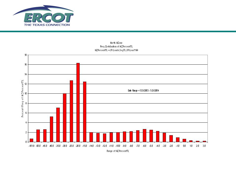
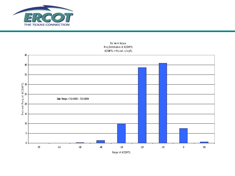
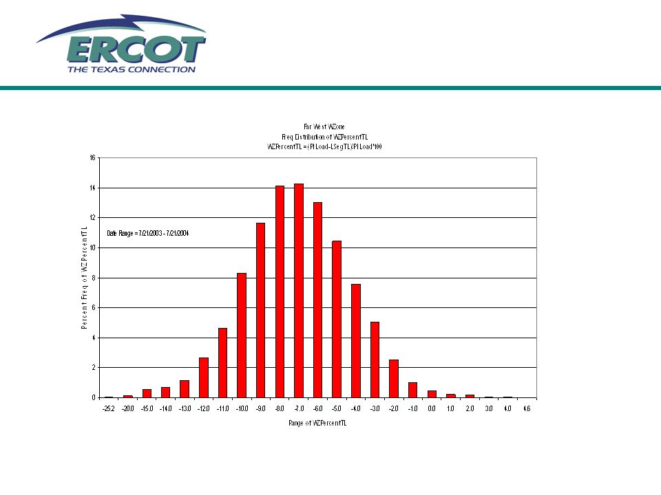
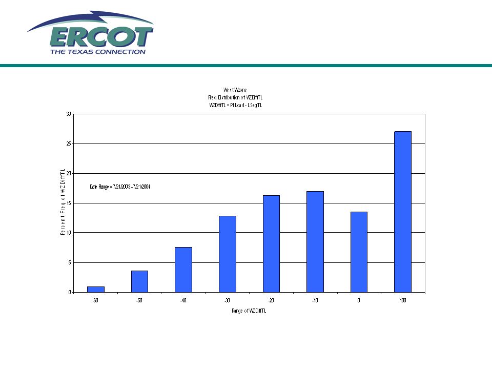
25. Frequency Analysis of UFE By Weather Zone

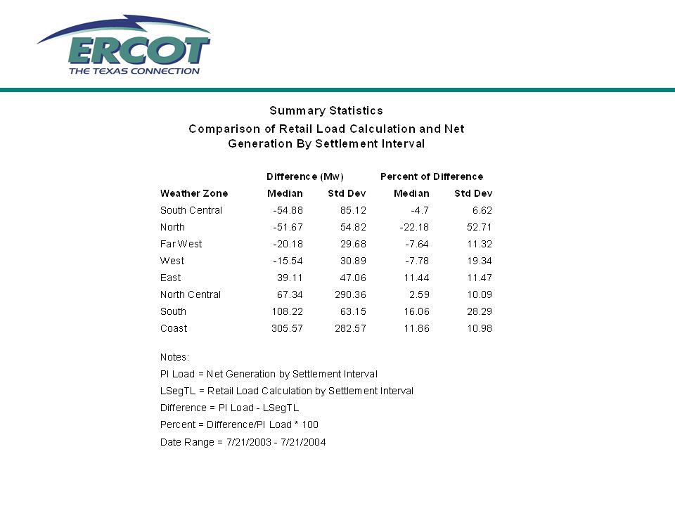
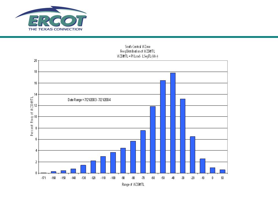
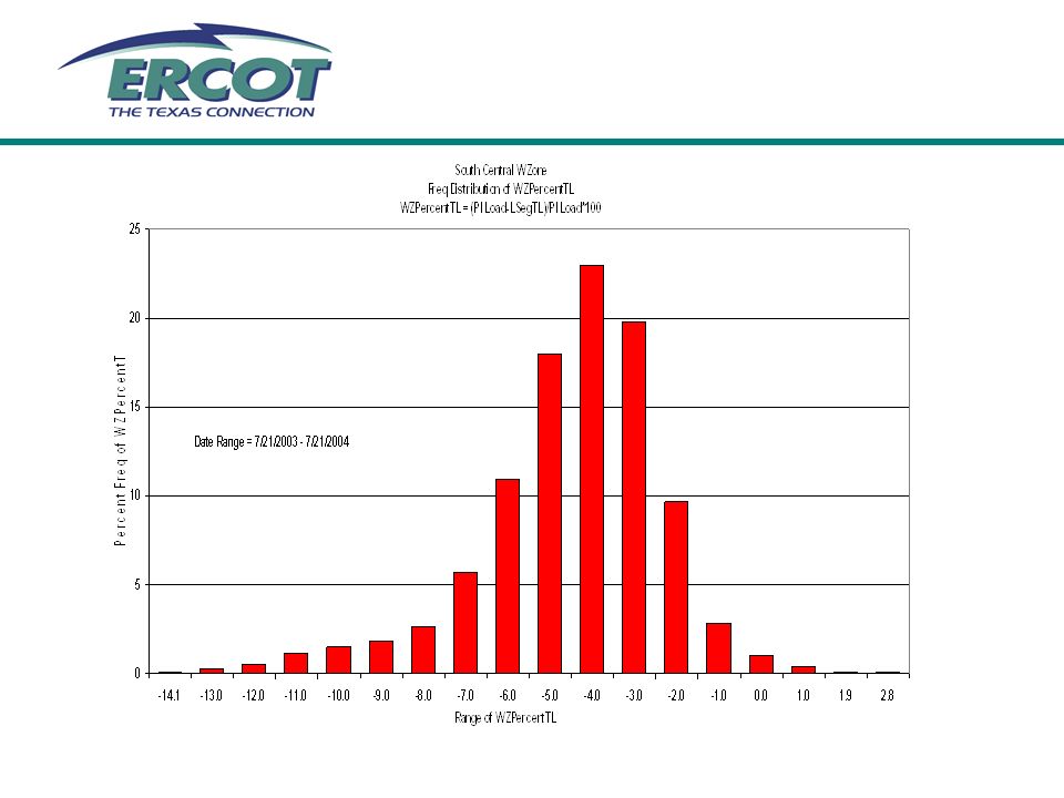
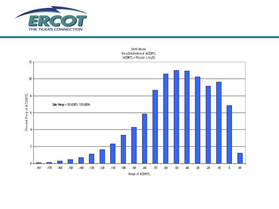
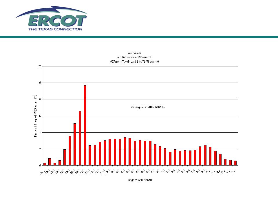
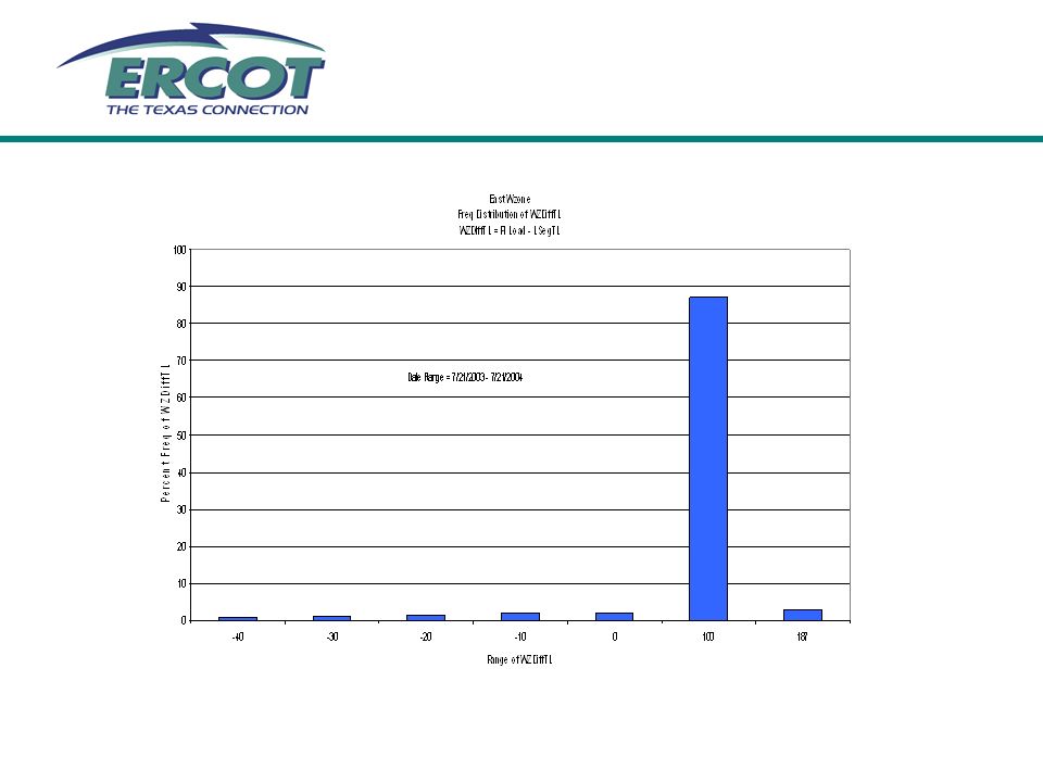
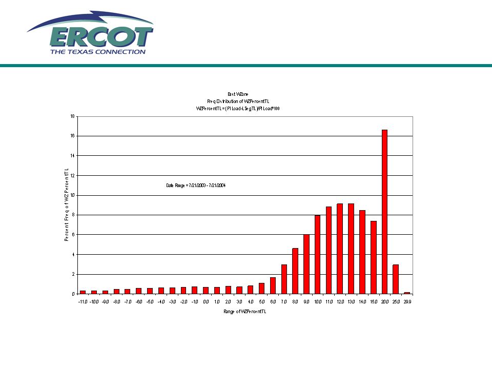
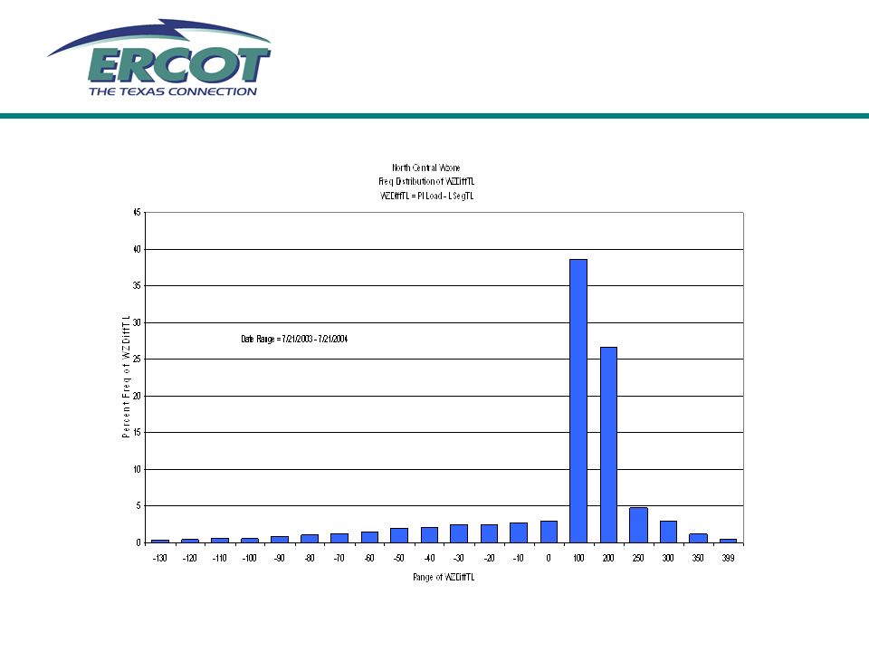
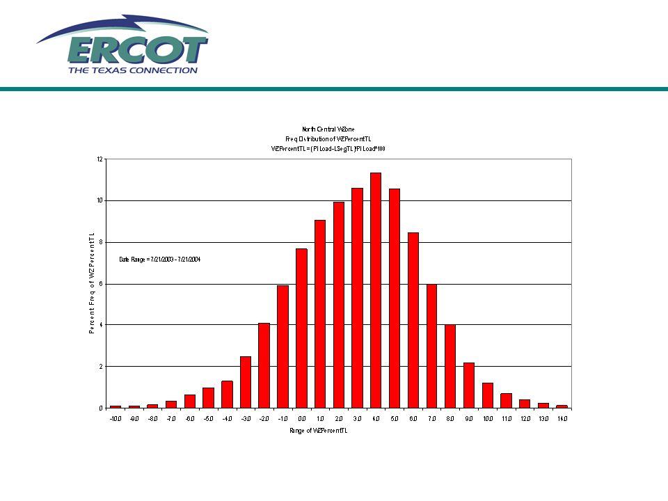
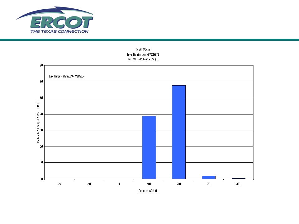
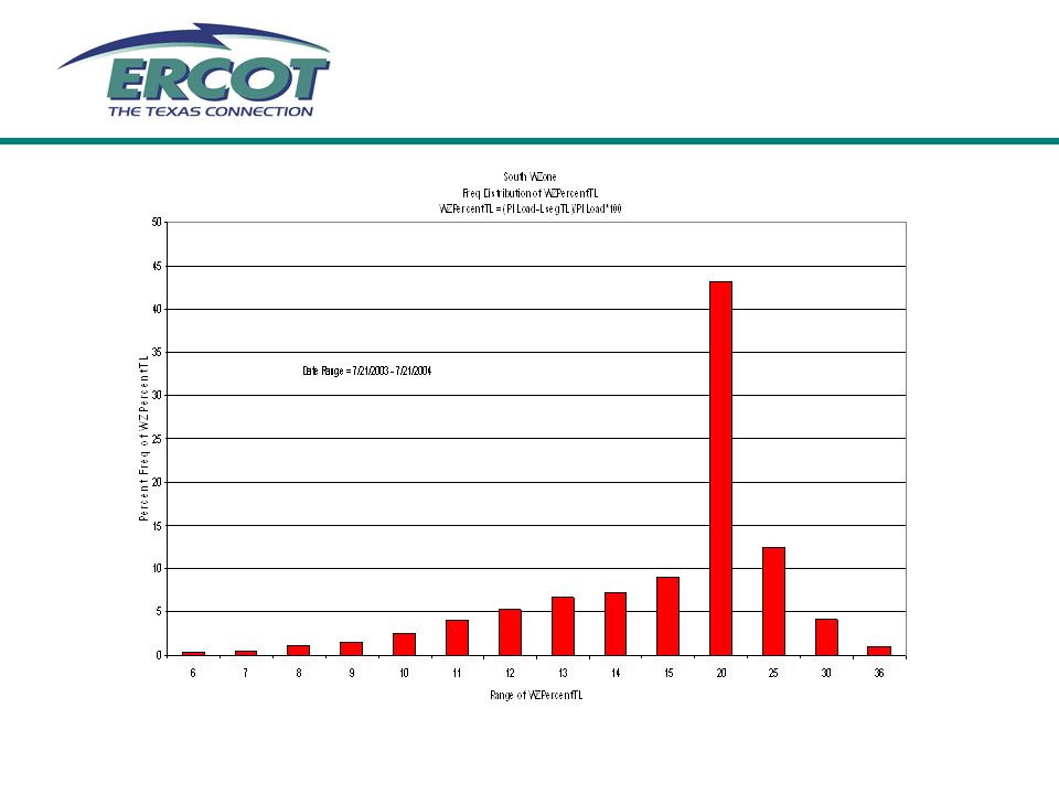
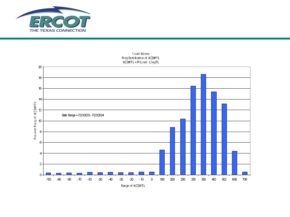
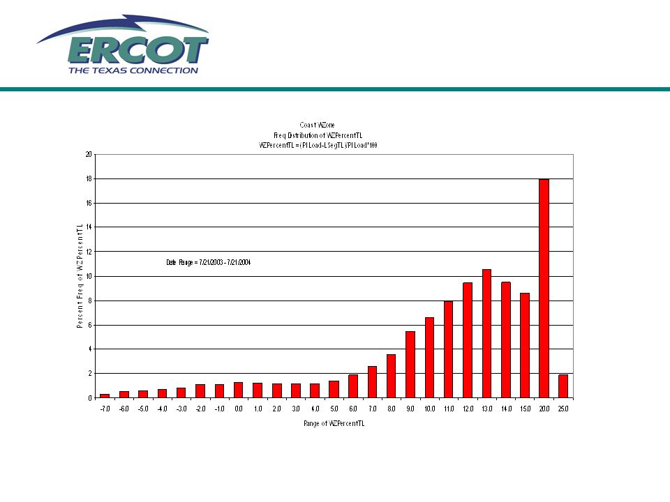
26. Frequency Analysis Study Definition Comparison of retail load build-up (LSegTL) with net load (generation) including actual losses LSegTL includes ESI ID Kwh + NOIE Kwh assigned to a Weather Zone because Operations data represents total load in Weather Zone Net_Load (PI_Load) by Weather Zone is calculated by operations as a small control area (∑Gen – ∑Interchange = Load) with generation and metering (interchange) points assigned to a Weather Zone Date Range: 7/21/2003 - 7/21/2004 Frequency plots are included for difference and percent of difference by Weather Zone Difference = (PI_Load – LSegTL) for each Settlement Interval Percent of Difference = Difference / PI_Load * 100

44. There is a significant bias (positive or negative) in the difference and percent of difference by Weather Zone Possible causes of the bias: –Weather Zone assignment of interchange (meter) points and generation used in the net load (generation) calculation –Weather Zone assignment of ESI ID’s used in the LSegTL calculation –Inaccurate transmission loss calculation or allocation –Inaccurate distribution loss calculation –Inaccurate profiles by weather zone Observations

45. UFE Allocation Should the current UFE allocation proportions be maintained?

46. UFE Allocation UFE is currently allocated with arbitrary weighting factors –0.10 - Distribution Voltage level IDR Non Opt-in Entities –0.10 - Transmission Voltage level IDR Premises –0.50 - Distribution Voltage level IDR Premises –1.00 - Distribution Voltage level Profiled Premises Alternatively could allocate UFE based on the category’s estimated load plus estimated loss IDRs settled with actual data would only be allocated UFE based on losses Profiled load and estimated IDRs would be allocated based on both load and loss Would have a different allocation factor in each interval

47. Hypothetical Example Based on July 12, 2004 at 13:45

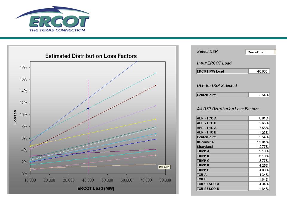
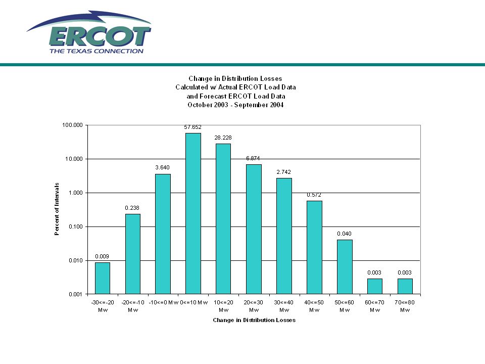
48. Distribution Loss Calculation PRR 565 is going through stakeholder approval Primary change is to base loss calculations on Actual Ercot System Load rather than the day ahead Should result in more accurate distribution loss estimates (and consequently have an effect on UFE) and use the same basis as is currently used for transmission losses

49. Examining the Calculations The distribution loss factors for a selected TDSP are calculated using the following formula: SILF i = ADLF * [K + (1 - K) * (SIEL i /AAL)] Where: i = Interval SILF = Settlement Interval Distribution Loss Factor ADLF = Annual Distribution Loss Factor (based on TDSP Loss Study) K = constant representing the no load loss factor (based on TDSP Loss Study) SIEL = Settlement Interval ERCOT Load (ERCOT Day Ahead Forecasted MW Load divided by 4) AAL = ERCOT Annual interval Average Load (ERCOT will use 8,073 MWh for year 2004 calculations) ADLF, K and AAL are all based on historical actual load … the most accurate application of the loss factor formula will be to base it on actual ERCOT load

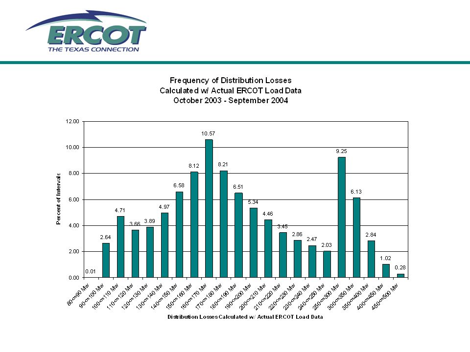
54. Statistics for Distribution Loss and UFE Calculations

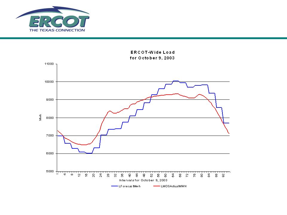
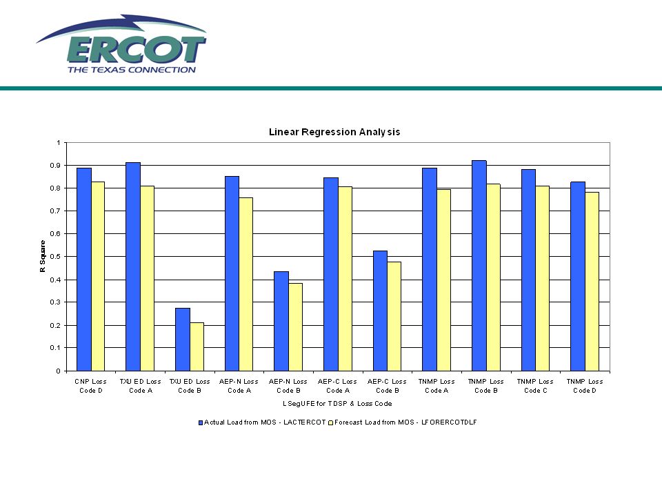
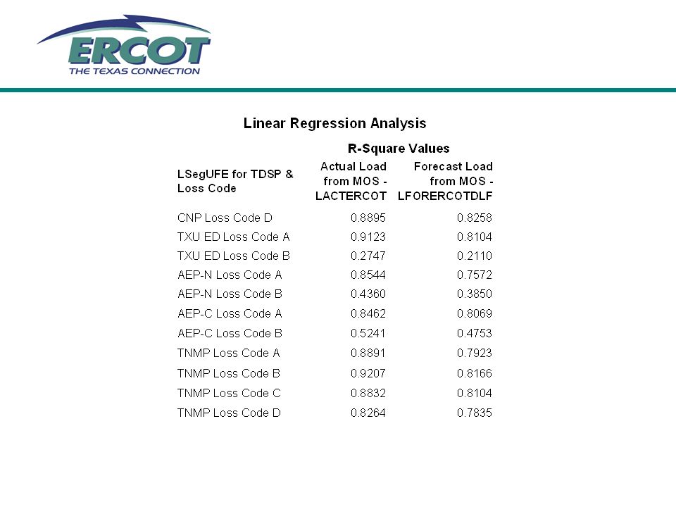
57. Distribution Loss Calculation Findings Forecast of ERCOT System Load contains error and is biased high Distribution loss calculations reflect the forecasting error/bias … distribution losses tend to be overstated TDSP losses are a function of the TDSP load; Actual ERCOT load has a stronger correlation to TDSP actual load than forecasted ERCOT load TDSP Loss Studies are based on actual TDSP and ERCOT loads … its more consistent to apply the DLFs produced by those studies to actual ERCOT load