Download presentation
Presentation is loading. Please wait.

1
How accurately do N body simulations reproduce the clustering of CDM? Michael Joyce LPNHE, Université Paris VI Work in collaboration with: T. Baertschiger (La Sapienza, Rome) A. Gabrielli (Istituto dei Sistemi Complessi-CNR, Rome) B. Marcos & F. Sylos Labini (Centro E. Fermi, Rome)
 A. Gabrielli (Istituto dei Sistemi Complessi-CNR, Rome) B. Marcos & F. Sylos Labini (Centro E. Fermi, Rome).")
2
Outline Intro: Theory vs. simulation or what is the problem? Qualitative expectations or is it a real problem? Systematic analytical approaches: (Initial conditions) Perturbative regime Towards control of the non-linear regime Comments on numerical testing Other approaches
 Perturbative regime Towards control of the non-linear regime Comments on numerical testing Other approaches.")
3
What is the problem? N body simulations are not a direct discretization of the theoretical equations of motion a “numerically perfect” simulation ≠ theory

4
What is the problem? Theory (What one would like to simulate) Purely self-gravitating microscopic particles (typically ~10 70 /[Mpc] 3 ) Treated statistically ---> Vlasov-Poisson equations for f(v,x,t) “Collisionless” (mean field) limit Fluid/continuum limit (appropriate N --> ) Physics: separation of scales scales of discrete “graininess” << scales of clustering
 Purely self-gravitating microscopic particles (typically ~10 70 /[Mpc] 3 ) Treated statistically ---> Vlasov-Poisson equations for f(v,x,t) Collisionless (mean field) limit Fluid/continuum limit (appropriate N --> ) Physics: separation of scales scales of discrete graininess << scales of clustering.")
5
What is the problem? N body systems (What is in fact simulated) Purely self-gravitating macroscopic particles (typically ~(1-100)/[Mpc] 3 ) Direct evolution under Newtonian self-gravity Expanding background + small scale smoothing on force
 Purely self-gravitating macroscopic particles (typically ~(1-100)/[Mpc] 3 ) Direct evolution under Newtonian self-gravity Expanding background + small scale smoothing on force.")
6
What is the problem? The discreteness (finite N) problem What is the relation between e.g. a correlation function or power spectrum calculated from output of an NBS and the same quantity in the theory? Answer: we don’t know ! Since theory is an appropriate N --> limit, the problem may be stated: what are the corrections due to the use of finite N ?

7
Is it really a problem? Is N ~ 10 10 (e.g. “Millenium”) not enough? Answer: it depends on what you want to resolve. Simulators systematically make very optimistic assumptions Surely simulators understand and control this? Answer: No! There are some (but very few) numerical studies. In general only qualitative arguments for trusting results are given.
 numerical studies. In general only qualitative arguments for trusting results are given..")
8
Is it really a problem? The issue of resolution Unphysical characteristic scales are introduced by the “discretization”: Interparticle separation l, force smoothing [and box size L, with N=(L/l) 3 ] Naively: fluid continuum limit for scales >> l In practice: results are taken as physical (usually) down to , where << l Why? This is the “interesting” regime (strongly non-linear)… e.g. “Millenium” simulation: l ≈ 0,25 h -1 Mpc, ≈ 5 h -1 kpc Is it justified? If so, what are errors?
 3 ] Naively: fluid continuum limit for scales >> l In practice: results are taken as physical (usually) down to , where << l Why. This is the interesting regime (strongly non-linear)… e.g. Millenium simulation: l ≈ 0,25 h -1 Mpc, ≈ 5 h -1 kpc Is it justified. If so, what are errors .")
9
Is it really a problem? Some common wisdom justifying this practice Numerical tests show that results are robust to changes in N (---> l) Some analytical “predictions” work well: notably Press-Schecter formalism Self-similar scaling for power law initial power spectra Physics: “transfer of power to small scales is very efficient”
 Some analytical predictions work well: notably Press-Schecter formalism Self-similar scaling for power law initial power spectra Physics: transfer of power to small scales is very efficient .")
10
Is it really a problem? Caveats to this common wisdom Numerical studies in the literature are few and unsystematic (other parameters varied --- see below), very limited range of l (at very most factor of 10, typically by 2) do not agree (e.g. Melott et al.conclude that extrapolation is not justified) Physics: PS, self-similarity --> structures form predominantly by collapse, with linear theory setting the appropriate mass/time scales. This does not establish validity of Vlasov/fluid description in non-linear regime. Important: N independence does not imply Vlasov!
, very limited range of l (at very most factor of 10, typically by 2) do not agree (e.g. Melott et al.conclude that extrapolation is not justified) Physics: PS, self-similarity --> structures form predominantly by collapse, with linear theory setting the appropriate mass/time scales. This does not establish validity of Vlasov/fluid description in non-linear regime. Important: N independence does not imply Vlasov!.")
11
Is it really a problem? So.. Our understanding of this fundamental issue about NBS is, at best, qualitative We need a “theory of discreteness errors” leading to: A physical understanding of these effects Methods for quantifying these effects (analytically or numerically)
.")
12
Rest of talk: A problem in three parts Initial conditions of simulations The perturbative regime (up to “shell-crossing”) The non-linear regime
 The non-linear regime")
13
Analytical approaches I Discreteness effects in initial conditions (IC) IC are generated by displacing particles off a lattice (or “glass”) using Zeldovich Approximation.
 IC are generated by displacing particles off a lattice (or glass ) using Zeldovich Approximation.")
14
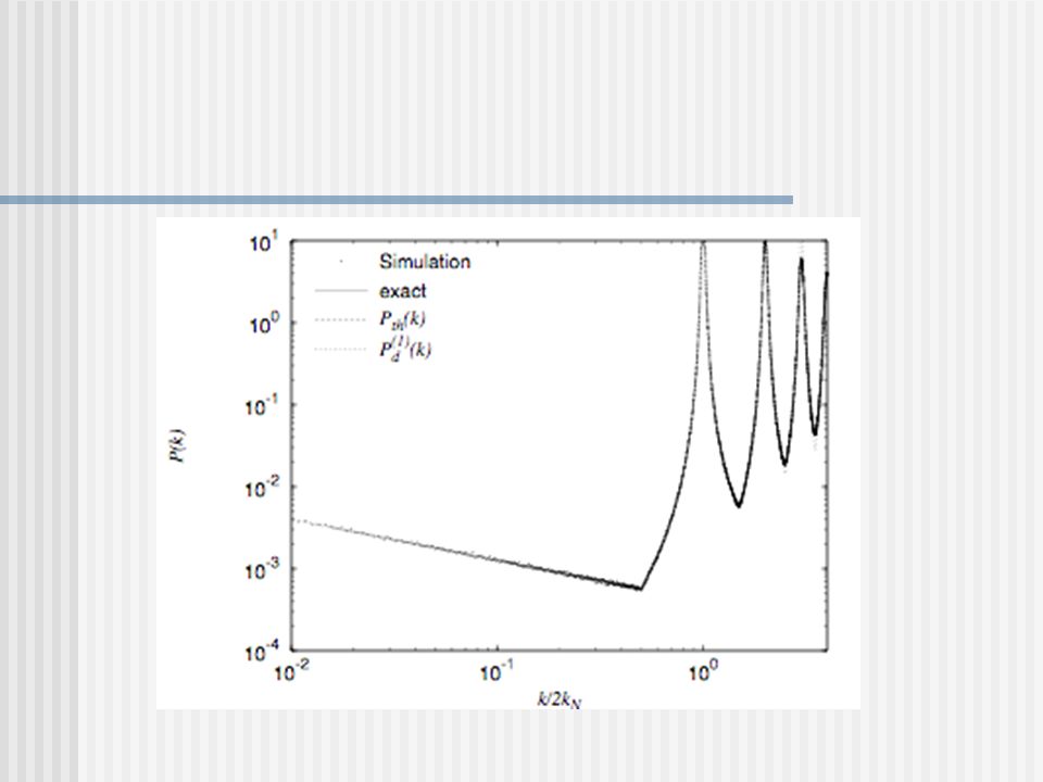
Input theoretical power spectrum Convolution term (linear in P th ) power spectrum of lattice (or glass) Analytical approaches I Full power spectrum of discrete IC
 power spectrum of lattice (or glass) Analytical approaches I Full power spectrum of discrete IC")
16
Theoretical correlation properties very well represented in reciprocal space for k k N In real space (e.g. mass variance) the relation is more complicated (discreteness terms are delocalized) ---> In the limit of low amplitude (i.e. high initial red-shift), at fixed N, the real space properties are not represented accurately Is this of dynamical importance? Analytical approaches I Conclusions on discreteness in IC
 the relation is more complicated (discreteness terms are delocalized) ---> In the limit of low amplitude (i.e. high initial red-shift), at fixed N, the real space properties are not represented accurately Is this of dynamical importance. Analytical approaches I Conclusions on discreteness in IC.")
17
Evolution of N body system can be solved perturbatively in displacements off the lattice Gives discrete generalisation of Lagrangian perturbative theory for fluid. ---> Recover the fluid limit and study N dependent corrections to it Analytical approaches II Perturbative treatment of the N body problem

18
Analytical approaches II Linearisation of the N body problem

19
Analytical approaches II Linear evolution of displacement fields

20
Analytical approaches II Eigenvalues for a simple cubic lattice

21
Analytical approaches II Growth of power in “particle linear theory”

22
Analytical approaches II Corrections in amplification due to discreteness Simulation begins at a=1 Deviation from unity is the discreteness effect

23
Analytical approaches II What we learn from this perturbative regime Fluid evolution for a mode k recovered for kl << 1 i.e. as naively expected. Exact fluid evolution is thus recovered by imposing a cut-off k C in the input power spectrum, and taking k C l --> 0 Discreteness effects in this regime accumulate in time. Taking initial red-shift z I --> , at fixed l, the simulation diverges from fluid (--> z I is a relevant parameter for discreteness!) These dynamical effects of discreteness are not two-body collision effects
 These dynamical effects of discreteness are not two-body collision effects.")
24
Not analytically tractable (that’s why we use simulations!) Need at least well defined numerical procedures to quantify discreteness Some approaches towards understanding physics: Detailed study of “simplified” simulations (e.g. “shuffled lattice”) Rigorous studies of simplified toy models (--> statistical physics of long range interactions) Towards control on the non-linear regime
 Rigorous studies of simplified toy models (--> statistical physics of long range interactions) Towards control on the non-linear regime.")
25
Increasing N to test for discreteness effects we should extrapolate towards the correct continuum limit. Formally it is N --> i.e. l --> 0 (in units of box size) What do we do with other relevant parameters: , z I, k C ? (Non-unique) answer: keep them fixed (in units of box size for , k C ) Note: For robust conclusions on NBS we need to extrapolate to l << k C -1 l large PM type simulations Towards control on the non-linear regime The continuum limit
 What do we do with other relevant parameters: , z I, k C . (Non-unique) answer: keep them fixed (in units of box size for , k C ) Note: For robust conclusions on NBS we need to extrapolate to l << k C -1 l large PM type simulations Towards control on the non-linear regime The continuum limit.")
26
Lattice with uncorrelated perturbations ( random error on positions) Power spectrum k 2 at small k Non-expanding space Findings: Self-similarity with temporal behaviour of fluid limit Form of non-linear correlation function already defined in nearest neighbour dominated (i.e. non-Vlasov) phase. N body “coarse-grainings” only converge in continuum limit (as above) Towards control on the non-linear regime Study of “shuffled lattices”
 phase. N body coarse-grainings only converge in continuum limit (as above) Towards control on the non-linear regime Study of shuffled lattices .")
27
N body simulators make very optimistic and rigorously unjustified assumptions about extrapolation to theory New formalism resolving the problem in the perturbative regime (--> defined continuum limit, quantifiable error, “correction” of IC) Physical effects of discreteness are more complex than two body collisionality + sampling in IC Numerical tests should extrapolate to continuum limit as defined. Other numerical and analytical approaches necessary. Conclusions

28
References M. Joyce, B. Marcos, A. Gabrielli, T. Baertschiger, F. Sylos Labini Gravitational evolution of a perturbed lattice and its fluid limit Phys. Rev. Lett. 95:011334(2005) B. Marcos, T. Baertschiger, M. Joyce, A. Gabrielli, F. Sylos Labini Linear perturbative theory of the discrete cosmological N body problem Phys.Rev. D73:103507(2006) M. Joyce and B. Marcos, Quantification of discreteness effects in cosmological N body simulations. I: Initial conditions Phys. Rev. D, in press,(2007) M. Joyce and B. Marcos, Quantification of discreteness effects in cosmological N body simulations. II: Early time evolution. In preparation (astro-ph soon) T. Baertschiger M. Joyce, A. Gabrielli, F. Sylos Labini Gravitational Dynamics of an Infinite Shuffled Lattice of Particles Phys.Rev. E, in press (2007) T. Baertschiger M. Joyce, A. Gabrielli, F. Sylos Labini Gravitational Dynamics of an Infinite Shuffled Lattice: Particle Coarse-grainings, Non-linear Clustering and the Continuum Limit, cond-mat/0612594
 B. Marcos, T. Baertschiger, M. Joyce, A. Gabrielli, F. Sylos Labini Linear perturbative theory of the discrete cosmological N body problem Phys.Rev. D73:103507(2006) M. Joyce and B. Marcos, Quantification of discreteness effects in cosmological N body simulations. I: Initial conditions Phys. Rev. D, in press,(2007) M. Joyce and B. Marcos, Quantification of discreteness effects in cosmological N body simulations. II: Early time evolution. In preparation (astro-ph soon) T. Baertschiger M. Joyce, A. Gabrielli, F. Sylos Labini Gravitational Dynamics of an Infinite Shuffled Lattice of Particles Phys.Rev. E, in press (2007) T. Baertschiger M. Joyce, A. Gabrielli, F. Sylos Labini Gravitational Dynamics of an Infinite Shuffled Lattice: Particle Coarse-grainings, Non-linear Clustering and the Continuum Limit, cond-mat/")
Similar presentations


 Korea Institute for Advanced Study ( ) Feb. 12 th.>")
 1. Introduction 2. Electromagnetic properties of the early universe 3. Magnetogenesis & tight coupling approximation.>")


>")


 Mona Berciu, UBC Collaborators: Glen Goodvin, George Sawaztky, Alexandru Macridin More.>")

-cosmology model Prado Martín Moruno IFF (CSIC) ERE2008 S. Capozziello, P. Martín-Moruno and C. Rubano.>")

![Macroscopic Behaviours of Palatini Modified Gravity Theories 0801.0603[gr-qc] and 0805.3428[gr-qc] Baojiu Li, David F. Mota & Douglas J. Shaw Portsmouth,](/16/5159565/big_thumb.jpg "Macroscopic Behaviours of Palatini Modified Gravity Theories 0801.0603[gr-qc] and 0805.3428[gr-qc] Baojiu Li, David F. Mota & Douglas J. Shaw Portsmouth,>")
 Nick Cowan UW Astronomy January 25, 2005.>")
