1. Chapter 6 – Three Simple Classification Methods © Galit Shmueli and Peter Bruce 2008 Data Mining for Business Intelligence Shmueli, Patel & Bruce

2. Methods & Characteristics The three methods: Naïve rule Naïve Bayes K-nearest-neighbor Common characteristics: Data-driven, not model-driven Make no assumptions about the data

3. Naïve Rule Classify all records as the majority class Not a “real” method Introduced so it will serve as a benchmark against which to measure other results

4. Naïve Bayes

5. Naïve Bayes: The Basic Idea For a given new record to be classified, find other records like it (i.e., same values for the predictors) What is the prevalent class among those records? Assign that class to your new record

6. Usage Requires categorical variables Numerical variable must be binned and converted to categorical Can be used with very large data sets Example: Spell check – computer attempts to assign your misspelled word to an established “class” (i.e., correctly spelled word)

7. Exact Bayes Classifier Relies on finding other records that share same predictor values as record-to-be-classified. Want to find “probability of belonging to class C, given specified values of predictors.” Even with large data sets, may be hard to find other records that exactly match your record, in terms of predictor values.

8. Solution – Naïve Bayes Assume independence of predictor variables (within each class) Use multiplication rule Find same probability that record belongs to class C, given predictor values, without limiting calculation to records that share all those same values

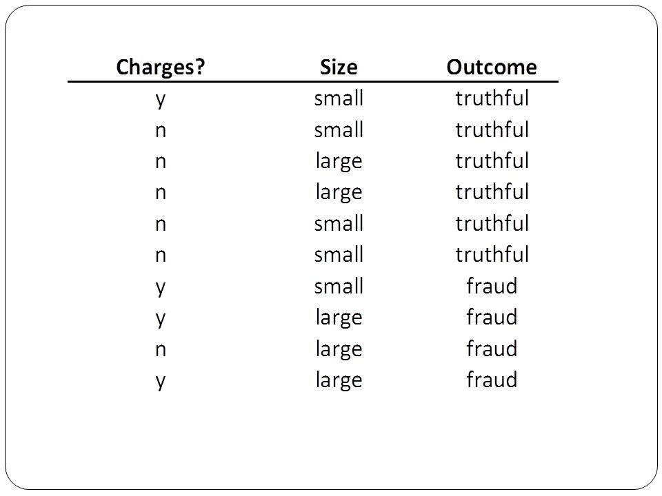
9. Example: Financial Fraud Target variable: Audit finds fraud, no fraud Predictors: Prior pending legal charges (yes/no) Size of firm (small/large)

11. Exact Bayes Calculations Goal: classify (as “fraudulent” or as “truthful”) a small firm with charges filed There are 2 firms like that, one fraudulent and the other truthful P(fraud|charges=y, size=small) = ½ = 0.50 Note: calculation is limited to the two firms matching those characteristics

12. Naïve Bayes Calculations Goal: Still classifying a small firm with charges filed Compute 2 quantities: Proportion of “charges = y” among frauds, times proportion of “small” among frauds, times proportion frauds = 3/4 * 1/4 * 4/10 = 0.075 Prop “charges = y” among frauds, times prop. “small” among truthfuls, times prop. truthfuls = 1/6 * 4/6 * 6/10 = 0.067 P(fraud|charges, small) = 0.075/(0.075+0.067) = 0.53

13. Naïve Bayes, cont. Note that probability estimate does not differ greatly from exact All records are used in calculations, not just those matching predictor values This makes calculations practical in most circumstances Relies on assumption of independence between predictor variables within each class

14. Independence Assumption Not strictly justified (variables often correlated with one another) Often “good enough”

15. Advantages Handles purely categorical data well Works well with very large data sets Simple & computationally efficient

16. Shortcomings Requires large number of records Problematic when a predictor category is not present in training data Assigns 0 probability of response, ignoring information in other variables

17. On the other hand… Probability rankings are more accurate than the actual probability estimates Good for applications using lift (e.g. response to mailing), less so for applications requiring probabilities (e.g. credit scoring)

18. K-Nearest Neighbors

19. Basic Idea For a given record to be classified, identify nearby records “Near” means records with similar predictor values X 1, X 2, … X p Classify the record as whatever the predominant class is among the nearby records (the “neighbors”)

20. How to Measure “nearby”? The most popular distance measure is Euclidean distance

21. Choosing k K is the number of nearby neighbors to be used to classify the new record k=1 means use the single nearest record k=5 means use the 5 nearest records Typically choose that value of k which has lowest error rate in validation data

22. Low k vs. High k Low values of k (1, 3 …) capture local structure in data (but also noise) High values of k provide more smoothing, less noise, but may miss local structure Note: the extreme case of k = n (i.e. the entire data set) is the same thing as “naïve rule” (classify all records according to majority class)

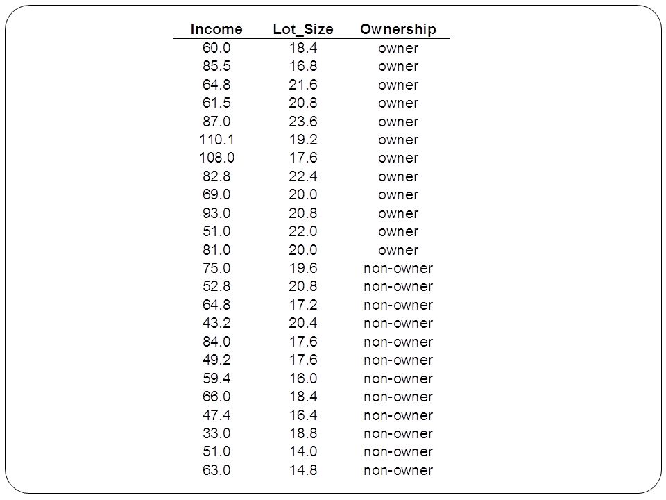
23. Example: Riding Mowers Data: 24 households classified as owning or not owning riding mowers Predictors = Income, Lot Size

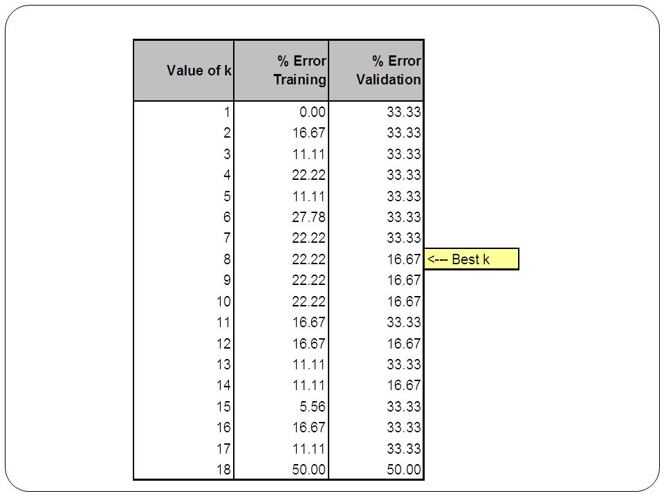
25. XLMiner Output For each record in validation data (6 records) XLMiner finds neighbors amongst training data (18 records). The record is scored for k=1, k=2, … k=18. Best k seems to be k=8. K = 9, k = 10, k=14 also share low error rate, but best to choose lowest k.

27. Using K-NN for Prediction (for Numerical Outcome) Instead of “majority vote determines class” use average of response values May be a weighted average, weight decreasing with distance

28. Advantages Simple No assumptions required about Normal distribution, etc. Effective at capturing complex interactions among variables without having to define a statistical model

29. Shortcomings Required size of training set increases exponentially with # of predictors, p This is because expected distance to nearest neighbor increases with p (with large vector of predictors, all records end up “far away” from each other) In a large training set, it takes a long time to find distances to all the neighbors and then identify the nearest one(s) These constitute “curse of dimensionality”

30. Dealing with the Curse Reduce dimension of predictors (e.g., with PCA) Computational shortcuts that settle for “almost nearest neighbors”

31. Summary Naïve rule: benchmark Naïve Bayes and K-NN are two variations on the same theme: “Classify new record according to the class of similar records” No statistical models involved These methods pay attention to complex interactions and local structure Computational challenges remain