1. Ice Investigation with PPC Dmitry Chirkin, UW (photon propagation code) http://icecube.wisc.edu/~dima/work/WISC/ppc/

2. AHA model AHA: method: de-convolve the smearing effect by using:  fits to the homogeneous ice (as in the ice paper)  un-smearing based on photonics weaknesses:  code used to fit the ice is not same as used in simulation  multiple photonics issues were discovered since the model was completed  photonics full-circle test demonstrates there are problems with ice description at all distance ranges  simulation based on this model does not agree with the: existing IceCube flasher (and standard candle?) data muon data neutrino data

3. Photonics full-circle test From http://wiki.icecube.wisc.edu/index.php/New_ice_model: All distancesNear: < 100 mFar: > 150 m If the layer smearing hypothesis is correct, the result from the fits should be (very close to) the millennium ice model (y2k). It is close only at near distances, up to a factor of 2 off at far distances

4. Fits with PPC PPC: method:  Direct fit of fully heterogeneous ice model to flasher data strengths:  code used to fit the ice is the same as used in simulation  simple procedure, using software based on ~800 lines of c++ code  ppc is bug-free: compared with photonics compared with Tareq’s i3mcml several different versions agree (c++, Assembly, GPU)  description of flasher data is much better than with AHA  describes muon background data (occupancy, COGz, etc)!  standard candle and neutrino data to be verified weaknesses:  slow

5. Using IceCube flasher data Chris Wendt pointed out that the waveforms obtained with hi- and low-P.E. data are of different width (likely reason being electronics smearing effects)  This is sometimes quoted as a reason that we need low-p.e. data to capture data that can be used to fit the ice properties correctly However, the total collected charge should be correct, less the saturation correction that becomes important above ~2000 p.e. (at 10 7 gain; by X. Bai, also see Chris Wendt and Patrick B. web pages on saturation)  most charges on the near strings are below ~500 p.e.  If that is too high, can go on to the strings farther away from flashers  Time profile before the pulse maximum is probably also correct

6. Large string-to-string variations Large string-to-string variations could be due to:  Direction of flashers relative to the observing strings  flasher-to-flasher variations in light output and width of pulse Average behavior can be obtained with < ~20% accuracy For the ice table fits it should also be possible to use the low-P.E. data that is planned to be collected. However,  the uncertainties on the light yield near flasher threshold are much higher, so probably only timing information can be used  Uncertainties in the flasher photon emission time profile are larger  cannot account for the HLC, so only SLC data is desired.

7. AHA (left) vs. PPC fit (right) Starting with average bulk ice after only 8 iterations with PPC: much better agreement at all depths Counterargument by Gary:  The slope in the tail is wrong Answer: the difference in slope between data and simulation is the same in both cases As explained on the previous pages, only the front of the pulse should be used in the fit The tails are derived from the FADC data, which could be off by up to a factor ~2 as shown by Tim Ruhe  however, FADC matched well to ATWD in the transition region (the dip) Differences up to factor ~10 in the AHA size (e.g., DOM ) are reduced to below ~20%.

8. Muons: AHA (left) vs. PPC fit (right)

9. Counterargument simulation does not propagate changes to ice model (stretching):  simplified simulation based on ppc does propagate these changes in a way consistent with expectation: http://icecube.wisc.edu/~dima/work/WISC/ppc/pics/ http://icecube.wisc.edu/~dima/work/WISC/ppc/pics/  Is the muon propagation at fault? this is too far-fetched this is irrelevant as the simulation based on AHA model does not agree with the IceCube flasher data  this statement is based on incorrectly-simulated photonics tables (discovered this week by Kotoyo)  ignore this argument until it is proven unambiguously This argument is irrelevant as means to claim no ice model based on fits to in-situ light sources can possibly ever fit the muon data.  The ice table base on PPC fits to flasher data yield excellent agreement of muon data and simulation

10. Stretched test with PPC nominal AHAstretched AHA

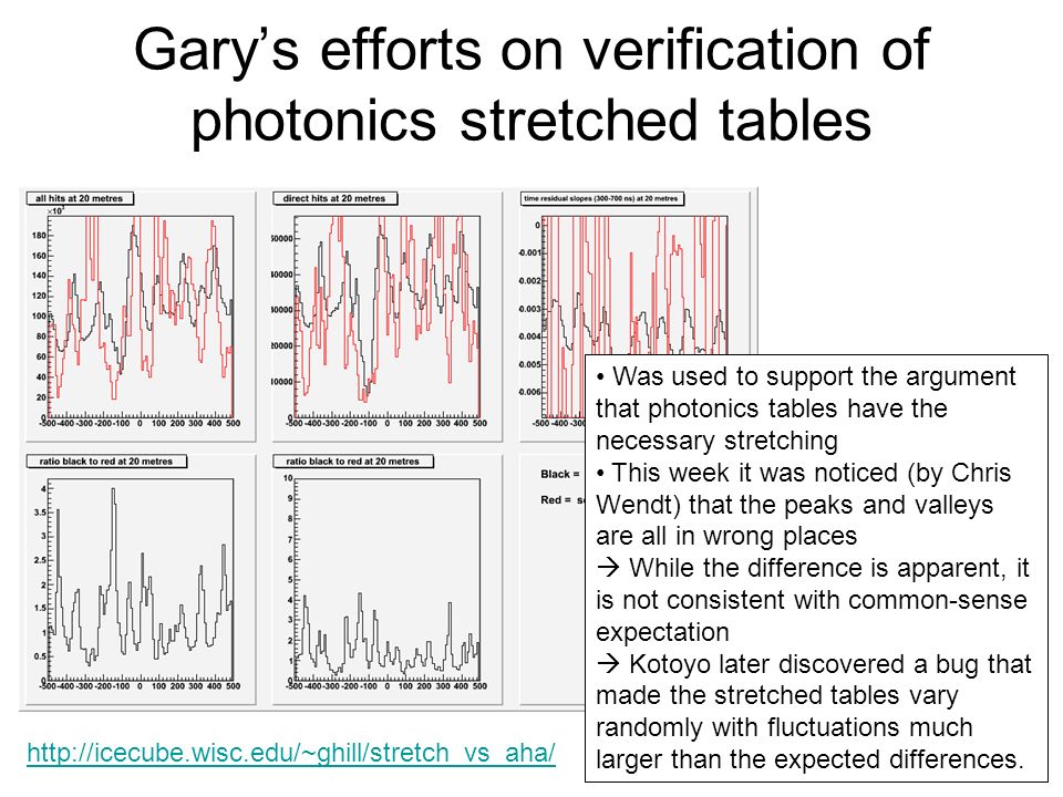
11. Gary’s efforts on verification of photonics stretched tables Was used to support the argument that photonics tables have the necessary stretching This week it was noticed (by Chris Wendt) that the peaks and valleys are all in wrong places  While the difference is apparent, it is not consistent with common-sense expectation  Kotoyo later discovered a bug that made the stretched tables vary randomly with fluctuations much larger than the expected differences. http://icecube.wisc.edu/~ghill/stretch_vs_aha/

12. Counterargument Still…, The likelihood profile of the a - e fit to the data (from the ice paper) is elongated along the direction of the a - e proportionality, thus much reducing the effects of “stretching” the ice model by modifying a and e by same amounts.

13. Another counterargument (by Gary) Won’t the new (different) ice properties contradict the AMANDA measurements? this was not proven some indications are that they won’t:  at near distances (< 100 m) nominal AHA and fit with PPC appear similar to each other Nominal AHAFit with PPC

14. Another counterargument … cont. Won’t the new (different) ice properties contradict the AMANDA measurements? Differences up to a factor ~2 are expected at 125 m, even higher in the dust layer (as p there is lower)! From Kurt’s page http://wiki.icecube.wisc.edu/index.php/Estimating_ice_systematics_in_UHE_analysis:http://wiki.icecube.wisc.edu/index.php/Estimating_ice_systematics_in_UHE_analysis

15. Calculation speed considerations For each iteration step: 10 9 photons generated for each DOM position (factor x 60)  takes ~4 hours on 40 nodes of npx2 (with the Assembly code) result shown above after 8 iterations (and a semi-empirical subjective correction after each step) What we want is a fully automatic procedure that varies scattering and absorption at 60 positions (120 parameters)  a speedup of 10 3 - 10 4 is desirable. this might be possible with running on a GPU  Tareq demonstrated 100x improvement compared to a single CPU node  PPC adaptation is in progress also reduce the number of generated photons (factor ~10) also further increase the DOM size (another factor ~10)

16. PPC in Assembly and PPC for GPU

17. Conclusions ice model based on fits to in-situ light sources can describe the muon data! fits to the flasher data with PPC are performed in one step, using same code that is used to verify other types of data (muons) fits with PPC are slow, so preliminary table is based on only 8 highly- subjective iterative steps. Faster version is being readied that will accelerate the calculation by ~1000x (a necessity for a fully-automated multi-ice-layer fit).