Download presentation
Presentation is loading. Please wait.

1
Benjamin Olken MIT Sampling and Sample Size

2
Course Overview 1.What is evaluation? 2.Measuring impacts (outcomes, indicators) 3.Why randomize? 4.How to randomize 5.Threats and Analysis 6.Sampling and sample size 7.RCT: Start to Finish 8.Cost Effectiveness Analysis and Scaling Up

3
Course Overview 1.What is evaluation? 2.Measuring impacts (outcomes, indicators) 3.Why randomize? 4.How to randomize 5.Threats and Analysis 6.Sampling and sample size 7.RCT: Start to Finish 8.Cost Effectiveness Analysis and Scaling Up

4
What’s the average result? If you were to roll a die once, what is the “expected result”? (i.e. the average)
.")
5
Possible results & probability: 1 die

6
Rolling 1 die: possible results & average

7
What’s the average result? If you were to roll two dice once, what is the expected average of the two dice?

8
Rolling 2 dice: Possible totals & likelihood

9
Rolling 2 dice: possible totals 12 possible totals, 36 permutations Die 1 Die 2 234567 345678 456789 5678910 6789 11 789101112

10
Rolling 2 dice: Average score of dice & likelihood

11
Outcomes and Permutations Putting together permutations, you get: 1.All possible outcomes 2.The likelihood of each of those outcomes –Each column represents one possible outcome (average result) –Each block within a column represents one possible permutation (to obtain that average) 2.5
 –Each block within a column represents one possible permutation (to obtain that average) 2.5")
12
Rolling 3 dice: 16 results 3 18, 216 permutations

13
Rolling 4 dice: 21 results, 1296 permutations

14
Rolling 5 dice: 26 results, 7776 permutations

15
Looks like a bell curve, or a normal distribution Rolling 10 dice: 50 results, >60 million permutations

16
>99% of all rolls will yield an average between 3 and 4 Rolling 30 dice: 150 results, 2 x 10 23 permutations*

17
>99% of all rolls will yield an average between 3 and 4 Rolling 100 dice: 500 results, 6 x 10 77 permutations

18
Rolling dice: 2 lessons 1.The more dice you roll, the closer most averages are to the true average (the distribution gets “tighter”) -THE LAW OF LARGE NUMBERS- 2.The more dice you roll, the more the distribution of possible averages (the sampling distribution) looks like a bell curve (a normal distribution) -THE CENTRAL LIMIT THEOREM-
 -THE LAW OF LARGE NUMBERS- 2.The more dice you roll, the more the distribution of possible averages (the sampling distribution) looks like a bell curve (a normal distribution) -THE CENTRAL LIMIT THEOREM-")
19
Which of these is more accurate? I. II. A. I. B. II. C. Don’t know

20
Accuracy versus Precision Precision (Sample Size) Accuracy (Randomization) truth estimates
 Accuracy (Randomization) truth estimates")
21
Accuracy versus Precision Precision (Sample Size) Accuracy (Randomization) truth estimates truth estimates
 Accuracy (Randomization) truth estimates truth estimates")
22
THE basic questions in statistics How confident can you be in your results? How big does your sample need to be?

23
THAT WAS JUST THE INTRODUCTION

24
Outline Sampling distributions –population distribution –sampling distribution –law of large numbers/central limit theorem –standard deviation and standard error Detecting impact

25
Outline Sampling distributions –population distribution –sampling distribution –law of large numbers/central limit theorem –standard deviation and standard error Detecting impact

26
Baseline test scores

27
Mean = 26

28
Standard Deviation = 20

29
Let’s do an experiment Take 1 Random test score from the pile of 16,000 tests Write down the value Put the test back Do these three steps again And again 8,000 times This is like a random sample of 8,000 (with replacement)
")
30
Good, the average of the sample is about 26… What can we say about this sample?

31
But… … I remember that as my sample goes, up, isn’t the sampling distribution supposed to turn into a bell curve? (Central Limit Theorem) Is it that my sample isn’t large enough?
 Is it that my sample isn’t large enough .")
32
This is the distribution of my sample of 8,000 students! Population v. sampling distribution

33
Outline Sampling distributions –population distribution –sampling distribution –law of large numbers/central limit theorem –standard deviation and standard error Detecting impact

34
How do we get from here… To here… This is the distribution of the population (Population Distribution) This is the distribution of Means from all Random Samples (Sampling distribution)
 This is the distribution of Means from all Random Samples (Sampling distribution)")
35
Draw 10 random students, take the average, plot it: Do this 5 & 10 times. Inadequate sample size No clear distribution around population mean

36
More sample means around population mean Still spread a good deal Draw 10 random students: 50 and 100 times

37
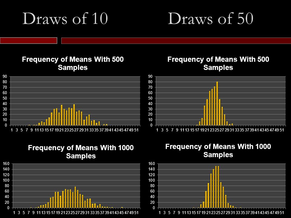
Distribution now significantly more normal Starting to see peaks Draws 10 random students: 500 and 1000 times

38
Draw 10 Random students This is like a sample size of 10 What happens if we take a sample size of 50?

39
N = 10 N = 50

40
Draws of 10 Draws of 50

42
Outline Sampling distributions –population distribution –sampling distribution –law of large numbers/central limit theorem –standard deviation and standard error Detecting impact

43
Population & sampling distribution: Draw 1 random student (from 8,000)
")
44
Sampling Distribution: Draw 4 random students (N=4)
")
45
Law of Large Numbers : N=9

46
Law of Large Numbers: N =100

47
The white line is a theoretical distribution Central Limit Theorem: N=1

48
Central Limit Theorem : N=4

49
Central Limit Theorem : N=9

50
Central Limit Theorem : N =100

51
Outline Sampling distributions –population distribution –sampling distribution –law of large numbers/central limit theorem –standard deviation and standard error Detecting impact

52
Standard deviation/error What’s the difference between the standard deviation and the standard error? The standard error = the standard deviation of the sampling distributions

53
Variance and Standard Deviation

54
Standard Deviation/ Standard Error

55
Sample size ↑ x4, SE ↓ ½

56
Sample size ↑ x9, SE ↓ ?

57
Sample size ↑ x100, SE ↓?

58
Outline Sampling distributions Detecting impact –significance –effect size –power –baseline and covariates –clustering –stratification

59
Baseline test scores

60
We implement the Balsakhi Program (lecture 3)
")
61
After the balsakhi programs, these are the endline test scores Endline test scores

62
The impact appears to be? A.Positive B.Negative C.No impact D.Don’t know

63
Stop! That was the control group. The treatment group is red. Post-test: control & treatment

64
Is this impact statistically significant? A.Yes B.No C.Don’t know Average Difference = 6 points

65
One experiment: 6 points

66
One experiment

67
Two experiments

68
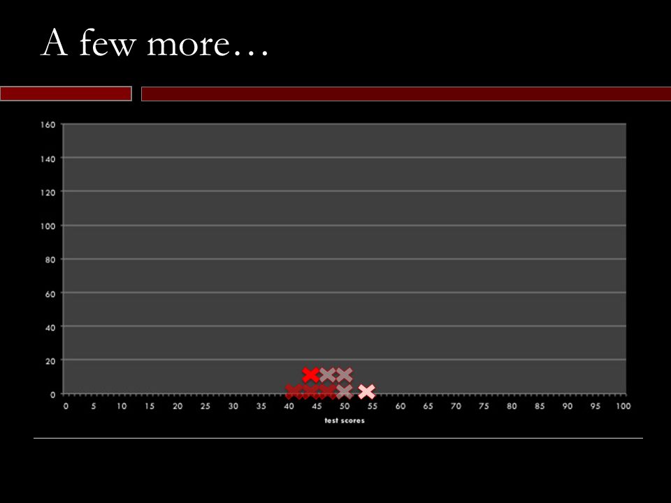
A few more…

70
Many more…

71
A whole lot more…

72
…

73
Running the experiment thousands of times… By the Central Limit Theorem, these are normally distributed

74
Hypothesis testing In criminal law, most institutions follow the rule: “innocent until proven guilty” The presumption is that the accused is innocent and the burden is on the prosecutor to show guilt –The jury or judge starts with the “null hypothesis” that the accused person is innocent –The prosecutor has a hypothesis that the accused person is guilty 74

75
Hypothesis testing In program evaluation, instead of “presumption of innocence,” the rule is: “presumption of insignificance” The “Null hypothesis” (H 0 ) is that there was no (zero) impact of the program The burden of proof is on the evaluator to show a significant effect of the program
 is that there was no (zero) impact of the program The burden of proof is on the evaluator to show a significant effect of the program")
76
Hypothesis testing: conclusions If it is very unlikely (less than a 5% probability) that the difference is solely due to chance: –We “reject our null hypothesis” We may now say: –“our program has a statistically significant impact”
 that the difference is solely due to chance: –We reject our null hypothesis We may now say: – our program has a statistically significant impact")
77
What is the significance level? Type I error: rejecting the null hypothesis even though it is true (false positive) Significance level: The probability that we will reject the null hypothesis even though it is true
 Significance level: The probability that we will reject the null hypothesis even though it is true.")
78
Hypothesis testing: 95% confidence YOU CONCLUDE EffectiveNo Effect THE TRUTH Effective Type II Error (low power) No Effect Type I Error (5% of the time) 78
 No Effect Type I Error (5% of the time) 78")
79
What is Power? Type II Error: Failing to reject the null hypothesis (concluding there is no difference), when indeed the null hypothesis is false. Power: If there is a measureable effect of our intervention (the null hypothesis is false), the probability that we will detect an effect (reject the null hypothesis)
, when indeed the null hypothesis is false. Power: If there is a measureable effect of our intervention (the null hypothesis is false), the probability that we will detect an effect (reject the null hypothesis).")
80
Assume two effects: no effect and treatment effect β Before the experiment H0H0 HβHβ

81
Anything between lines cannot be distinguished from 0 Impose significance level of 5% HβHβ H0H0

82
Shaded area shows % of time we would find Hβ true if it was Can we distinguish Hβ from H0 ? HβHβ H0H0

83
What influences power? What are the factors that change the proportion of the research hypothesis that is shaded—i.e. the proportion that falls to the right (or left) of the null hypothesis curve? Understanding this helps us design more powerful experiments 83
 of the null hypothesis curve. Understanding this helps us design more powerful experiments 83.")
84
Power: main ingredients 1.Effect Size 2.Sample Size 3.Variance 4.Proportion of sample in T vs. C 5.Clustering

85
Power: main ingredients 1.Effect Size 2.Sample Size 3.Variance 4.Proportion of sample in T vs. C 5.Clustering

86
Effect Size: 1*SE Hypothesized effect size determines distance between means 1 Standard Deviation HβHβ H0H0

87
Effect Size = 1*SE H0H0 HβHβ

88
The Null Hypothesis would be rejected only 26% of the time Power: 26% If the true impact was 1*SE… HβHβ H0H0

89
Bigger hypothesized effect size distributions farther apart Effect Size: 3*SE 3*SE

90
Bigger Effect size means more power Effect size 3*SE: Power= 91% H0H0 HβHβ

91
What effect size should you use when designing your experiment? A.Smallest effect size that is still cost effective B.Largest effect size you estimate your program to produce C.Both D.Neither

92
Let’s say we believe the impact on our participants is “3” What happens if take up is 1/3? Let’s show this graphically Effect size and take-up

93
Let’s say we believe the impact on our participants is “3” Effect Size: 3*SE 3*SE

94
Take up is 33%. Effect size is 1/3rd Hypothesized effect size determines distance between means 1 Standard Deviation HβHβ H0H0

95
Take-up is reflected in the effect size Back to: Power = 26% HβHβ H0H0

96
Power: main ingredients 1.Effect Size 2.Sample Size 3.Variance 4.Proportion of sample in T vs. C 5.Clustering

97
By increasing sample size you increase… A.Accuracy B.Precision C.Both D.Neither E.Don’t know

98
Power: Effect size = 1SD, Sample size = N

99
Power: Sample size = 4N

100
Power: 64%

101
Power: Sample size = 9

102
Power: 91%

103
Power: main ingredients 1.Effect Size 2.Sample Size 3.Variance 4.Proportion of sample in T vs. C 5.Clustering

104
What are typical ways to reduce the underlying variance A.Include covariates B.Increase the sample C.Do a baseline survey D.All of the above E.A and B F.A and C

105
Variance There is sometimes very little we can do to reduce the noise The underlying variance is what it is We can try to “absorb” variance: –using a baseline –controlling for other variables In practice, controlling for other variables (besides the baseline outcome) buys you very little
 buys you very little")
106
Power: main ingredients 1.Effect Size 2.Sample Size 3.Variance 4.Proportion of sample in T vs. C 5.Clustering

107
Sample split: 50% C, 50% T H0H0 HβHβ

108
Power: 91%

109
If it’s not 50-50 split? What happens to the relative fatness if the split is not 50-50. Say 25-75?

110
Sample split: 25% C, 75% T H0H0 HβHβ

111
Power: 83%

112
Allocation to T v C

113
Power: main ingredients 1.Effect Size 2.Sample Size 3.Variance 4.Proportion of sample in T vs. C 5.Clustering

114
Clustered design: intuition You want to know how close the upcoming national elections will be Method 1: Randomly select 50 people from entire Indian population Method 2: Randomly select 5 families, and ask ten members of each family their opinion 114

115
Low intra-cluster correlation (Rho)
")
116
HIGH intra-cluster correlation (rho)
")
117
All uneducated people live in one village. People with only primary education live in another. College grads live in a third, etc. Rho on education will be.. A.High B.Low C.No effect on rho D.Don’t know

118
If rho is high, what is a more efficient way of increasing power? A.Include more clusters in the sample B.Include more people in clusters C.Both D.Don’t know

119
Testing multiple treatments ←0.15 SD→ ↖ 0.25 SD ↘ ↑ 0.15 SD ↓ ↑ 0.10 SD ↓ ←0.10 SD→ ↗ 0.05 SD ↙ 50 100 200

120
END

Similar presentations

 Example: Suppose you have the hypothesis that UW undergrads have higher than the average IQ.>")


: Alternative Hypothesis (H 1 ): a statistical analysis used to decide which of two competing.>")


