Download presentation
Presentation is loading. Please wait.

1
Spatial Analysis Part 1 This is probably a 2-day lecture and the most challenging one we’ve had ASK questions! We’ll get as far as we can today and resume where we left off on Monday

2
Spatial Analysis What is spatial analysis?
It is the means by which we turn raw geographic data into useful information It does so by adding greater informative content and value Spatial analysis reveals patterns, trends, and anomalies that might otherwise be missed It provides a check on human intuition It allows for analysis of data that could never be done by humans

3
Spatial Analysis Analysis is considered spatial if the results depend on the locations of the objects being analyzed. Thus if you move the objects, the results of spatial analyses will change. Spatial analyses generally requires both attributes and locations of objects.

4
Steps in Spatial Analysis
Frame the question we wish to ask. Find appropriate data to answer the question. Choose an analytical method appropriate to answer question. Process the data using the chosen method. Interpret the results of the analysis.

5
Spatial Relationships are at the Core of Spatial Analysis
Most spatial analyses are based on topological relationships: How near is Feature A to Feature B What features contain other features? What features are adjacent to other features? What features are connected to other features? From these topological building blocks, we can develop all sorts of spatial analysis approaches to answer many complex questions

6
Types of Spatial Analysis
We will consider six categories of spatial analyses: Queries (today) Measurements (today) Transformations (today) Descriptive summaries (next lecture) Optimization (next lecture) Hypothesis testing (next lecture)
 Measurements (today) Transformations (today) Descriptive summaries (next lecture) Optimization (next lecture) Hypothesis testing (next lecture)")
7
1. Queries Queries Attribute based Example: show me all pixels in a raster image with BV > 80. Location based List all the block groups that fall within Orange County A GIS can respond to queries by selecting the appropriate data in: A map view A table Both
![]()
8
The Map View Queries can be performed through interaction with a GIS on-screen map Identify objects Query data objects based on specific criteria of attributes Find coordinates of objects

9
The Table View Queries can be performed through interaction with a table Attribute based queries can be performed in the table. When objects are selected in a table, a GIS can automatically highlight the selected data objects in the map view, and vice versa.

10
2. Measurements Measure: Distance between two points Area of a polygon
Distances can be summed Example: a truck makes multiple stops on a route. What is the total distance traveled on the route? Other mathematical operations can be applied to distances: We can square a set of distances, add them up, divide by the amount of distances calculated in the set, and take the square root. What is an example of when this operation is used? Area of a polygon Example: What is the area of a preserved forest tract?

11
Measurement of Length Types of length measurements
Euclidean Distance: straight-line distance between two points on a flat plane (as the crow flies) Manhattan Distance: limits movement to orthogonal directions Great Circle Distance: the shortest distance between two points on the globe Network Distance: Along roads Along pipe network Along electric grid Along phone grid By river channels
 Manhattan Distance: limits movement to orthogonal directions. Great Circle Distance: the shortest distance between two points on the globe. Network Distance: Along roads. Along pipe network. Along electric grid. Along phone grid. By river channels.")
12
Euclidean Distance P2 (x2,y2) (x1 – x2)2 + (y1 – y2)2 C= C P1 (x1,y1)
Distances can be calculated between points, along lines, or in a variety of fashions with areas Euclidean Distance – is calculated in a Cartesian frame of reference: P2 (x2,y2) (x1 – x2)2 + (y1 – y2)2 C= C P1 (x1,y1) On what scales is this valid? Can we use this with latitude and longitude?
 (x1 – x2)2 + (y1 – y2)2. C= C. P1 (x1,y1) On what scales is this valid Can we use this with latitude and longitude")
13
Manhattan Distance P2 (x2,y2) dm = | x1 – x2 | + | y1 – y2 |
Manhattan Distance is useful in some urban environments with orthogonal road networks. Movement is limited to city streets: P2 (x2,y2) dm = | x1 – x2 | + | y1 – y2 | a reminder – the | symbols denote absolute value P1 (x1,y1)
 dm = | x1 – x2 | + | y1 – y2 | a reminder – the | symbols denote absolute value. P1 (x1,y1)")
14
Great Circle Distance The Great Circle distance is the shortest distance between two points on the globe. The two points must be specified using geographic coordinates (i.e., latitude & longitude positions).
.")
15
Great Circle Distance Calculating the great circle distance is actually pretty complicated A = Latitude of point A B = Latitude of point B C = Difference in longitude between the points (i.e., Longitude of point A – Longitude of point B) D = angular distance Simple version (spherical distance) cos(D) = sin(A) sin(B) + cos(A) cos(B) cos(C)
 D = angular distance. Simple version (spherical distance) cos(D) = sin(A) sin(B) + cos(A) cos(B) cos(C)")
16
Great Circle Distance ONE more complicated version (also more accurate) To use these equations: Convert latitude and longitude (degree, minute, second) to decimal degrees (if necessary) Convert degrees to into radians Solve the equation for D Great Circle Distance = D * the radius of the earth ( km) OR Convert D into degrees Great Circle Distance = D * length of 1 degree at the equator ( km)
 to decimal degrees (if necessary) Convert degrees to into radians. Solve the equation for D. Great Circle Distance = D * the radius of the earth ( km) OR. Convert D into degrees. Great Circle Distance = D * length of 1 degree at the equator ( km)")
17
Network Distance Yahoo maps:
Starting from: Carrboro, NC Save Address Arriving at: Washington, DC Save Address istance:272.5 miles Approximate Travel Time:5 hours 23 mins

18
Issues with Length Measurement
The length of a true curve is longer than the length of its polyline or polygon representation:

19
Issues with Length Measurement
Length measurements in GIS are usually calculated in 2 dimensions. But changes in elevation increase distances. X Z

20
3. Transformations Spatial transformations includes many analytical approaches, applicable to: Vector data Raster data Both Transformations can create new: Attributes Data objects

21
Buffering (Proximity Analysis)
Buffering operations create new objects consisting of areas within a user-defined distance of existing objects. Examples of uses: to determine areas impacted by a proposed highway to determine the service area of a proposed hospital Buffering can be performed in both the vector and raster spatial data models

22
Buffering (Proximity Analysis)
Buffering: The delineation of a zone around the feature of interest within a given distance. For a point feature, it is simply a circle with its radius equal to the buffer distance:

23
Variable Distance Buffering
The buffer zone constructed around each feature can be based on a variable distance according to some feature attribute(s) Suppose we have a point pollution source, such as a power plant. We want to zone residential areas some distance away from each plant, based on the amount of pollution that power plant produces For smaller power plants, the distance might be shorter. For larger power plants that generate a lot of pollutant, we choose longer distances
 Suppose we have a point pollution source, such as a power plant. We want to zone residential areas some distance away from each plant, based on the amount of pollution that power plant produces. For smaller power plants, the distance might be shorter. For larger power plants that generate a lot of pollutant, we choose longer distances.")
24
Buffering Points, Lines, and Polygons
Buffering higher order objects involves moving a circle of specified radius along the line (or the lines forming polygon)
")
25
Line and Polygon Buffer Examples
Buffer lines Buffer polygons

26
Raster Buffering Buffering operations also can be performed using the raster data model In the raster model, we can perform a simple distance buffer, or in this case, a distance buffered according to values in a friction layer (e.g. travel time for a bear through different landcover): lake Areas reachable in 5 minutes Areas reachable in 10 minutes Other areas
: lake. Areas reachable in 5 minutes. Areas reachable in 10 minutes. Other areas.")
27
Feature in Feature Transformations
These transformations determine whether a feature lies inside or outside of another feature The most basic of these transformations is point in polygon analysis, which can be applied in various situations:

28
The Point in Polygon Algorithm
How do GIS programs calculate this? Draw a line from the point to infinity in any direction, and then count the number of intersections between this line and each polygon’s boundary The polygon with an odd number of intersections is the containing polygon; all other polygons have an even number of intersections

29
Point in Polygon Algorithm
For the point to be inside the polygon, there must be an odd number of intersections on either side of the point .

30
Point Frequency/Density Analysis
We can use point in polygon results to calculate frequencies or densities of points per area For example, given a point layer of bird’s nests and polygon layer of habitats, we can calculate densities: Bird’s Nests A B D C Habitat Types A B D C Analysis Results Habitat Area(km2) Frequency Density A nests/km2 B nests/km2 C nests/km2 D nests/km2
 Frequency Density . A nests/km2. B nests/km2. C nests/km2. D nests/km2.")
31
Line in Polygon Analysis
Overlay line layer (A) with polygon layer (B) In which B polygons are A lines located? Assign polygon attributes from B to lines in A Example: Assign land use attributes (polygons) to streams (lines): A B David Tenenbaum – GEOG 070 – UNC-CH Spring 2005
 with polygon layer (B) In which B polygons are A lines located Assign polygon attributes from B to lines in A. Example: Assign land use attributes (polygons) to streams (lines): A. B. David Tenenbaum – GEOG 070 – UNC-CH Spring")
32
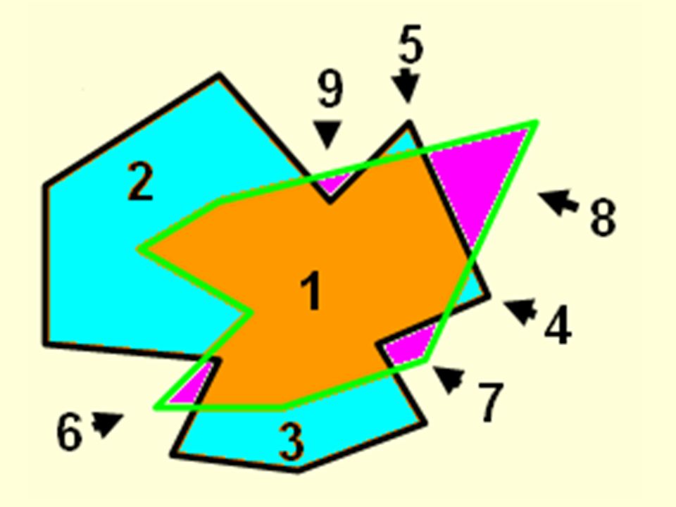
Polygon Overlay, Discrete Object Case
In this example, two polygons are intersected to form nine new polygons. One is formed from both input polygons (1); four are formed by Polygon A and not Polygon B (2-5); four are formed by Polygon B and not Polygon A (6-9) B A 5 9 2 8 1 4 7 6 3
; four are formed by Polygon A and not Polygon B (2-5); four are formed by Polygon B and not Polygon A (6-9) B. A")
34
Boolean Operations Boolean operations of OR & AND correspond to UNION & INTERSECTION, used in vector-based analyses A B OR UNION A B AND INTERSECTION We can apply these concepts in the raster spatial data model, when two input layers contain true/false or 1/0 data:

35
Polygon Combination B A 5 9 2 8 1 4 7 6 3
Common ways to combine polygons: Show all new polygons as in diagram. UNION (Boolean OR) INTERSECTION (Boolean AND) B A 5 9 2 8 1 4 7 6 3
 INTERSECTION (Boolean AND) B. A")
36
Boolean Operations with Raster Layers
The AND operation requires that the value of cells in both input layers be equal to 1 for the output to have a value of 1: 1 1 AND = The OR operation requires that the value of a cells in either input layer be equal to 1 for the output to have a value of 1: 1 1 OR =

37
Problems with Vector Overlay Analysis (esp. Polygon)
There is a tradeoff between the complexity and interpretability of results Complex input layers with many polygons can result in many more polygon combinations… can we make sense of all those combinations?

38
Problems with Vector Overlay Analysis (esp. Polygon)
Overlay analysis using the vector spatial data model is highly computationally intensive Complicated input layers can tax even current processors For example With 2 partially overlapping polygons (U & V) we can have 8 options: Neither U V U AND V U OR V U NOT V V NOT U V XOR U
 we can have 8 options: Neither. U. V. U AND V. U OR V. U NOT V. V NOT U. V XOR U.")
39
Problems with Vector Overlay Analysis (esp. Polygon)
For example With 3 (X, Y, & Z) partially overlapping polygons we can have many more options Any guesses for how many? There are 121 possible combinations! Just think of what this means for a dataset with even a few hundred polygons… this is what we mean by “computationally intensive” The graphic shows just a few simple ones
 partially overlapping polygons we can have many more options. Any guesses for how many There are 121 possible combinations! Just think of what this means for a dataset with even a few hundred polygons… this is what we mean by computationally intensive The graphic shows just a few simple ones.")
40
Problems with Vector Overlay Analysis (esp. Polygon)
There are often spatial mismatches between input layers Overlay can result in spurious sliver polygons We can “filter” out spurious slivers by querying to select all polygons with AREA less than some minimum threshold It is difficult to choose a threshold to avoid deleting ‘real’ polygons

41
Algebraic Operations w/ Raster Layers
We can extend this concept from Boolean logic to algebra Map algebra: Each cell is a number Mathematical operations are using the raster layers as input Calculations are done on a cell-by-cell basis The result for each cell is placed in a new raster layer. Suitability analysis example: Multiple raster input layers determine suitable sites: The cell values (attributes) in each raster layer represent ‘scores’. Raster layers are weighted based on their importance. Output scores are the sum of the input raster layers.
 in each raster layer represent ‘scores’. Raster layers are weighted based on their importance. Output scores are the sum of the input raster layers.")
42
Simple Arithmetic Operations
1 + = 2 Summation 1 = Multiplication 1 + = 3 2 Summation of more than two layers Near the mall Near work Near friend’s house Good place to live?

43
Raster Difference (Subtraction)
5 1 7 6 3 4 2 - = -2 -1 -3 The difference between two layers: One application for subtraction between layers is a simple image change detection: Example: Imagine you have 2 images of the same forest, 10 years apart. Question: How can the locations where substantial changes have occurred (i.e., logging or regrowth) be identified using the two images? Answer: To measure forest growth or logging, you can take the difference in reflected Near InfraRed (NIR) light between image dates. More infrared light = more chlorophyll and more vegetation
 be identified using the two images Answer: To measure forest growth or logging, you can take the difference in reflected Near InfraRed (NIR) light between image dates. More infrared light = more chlorophyll and more vegetation.")
44
Raster Division Questions: Can we perform the following operation?
Are there any circumstances where we cannot perform this operation? =

45
More Complex Operations
2 3 5 1 4 + = * a b c As with other algebra, where you put the parentheses makes a difference

46
Applying a Model to Our Data
Map algebra can also be applied in the context of computing a statistical linear regression What you probably learned in geometry: Y = a + bX, X is the explanatory (independent) variable Y is the dependent variable. The slope of the line is b and a is the intercept (the value of y when x = 0) Linear regression uses the same basic idea: Y = B0 + B1X1 + B2X2 + random error The B values are the coefficients The X values are the independent variables (2 in this case) For example maybe we sampled some forested field sites and generated the following equation: LAI = B0 + B1NDVI + B2TMI Using the coefficients we derived (the B values) we can apply the equation to our entire study area
 variable. Y is the dependent variable. The slope of the line is b and a is the intercept (the value of y when x = 0) Linear regression uses the same basic idea: Y = B0 + B1X1 + B2X2 + random error. The B values are the coefficients. The X values are the independent variables (2 in this case) For example maybe we sampled some forested field sites and generated the following equation: LAI = B0 + B1NDVI + B2TMI. Using the coefficients we derived (the B values) we can apply the equation to our entire study area.")
47
Making Inferences from Samples
Imagine that you have point location data, but you want data for your whole site/region. For example: Air temperature maps created from point data. Water pollution levels measured at points. Use models to predict values between sampling points Extrapolation: Predicting missing values using existing values that exist only on one side of the point in question Interpolation: Predicting unknown values using known values occurring at locations around the unknown value

48
Spatial Interpolation: Inverse Distance Weighting (IDW)
The unknown value at a point is estimated by taking a weighted average of known values Those known points closer to the unknown point have higher weights. Those known points farther from the unknown point have lower weights.

49
Sample weighting function
Spatial Interpolation: Inverse Distance Weighting (IDW) point i known value zi distance di weight wi unknown value (to be interpolated) at location x The estimate of the unknown value is a weighted average Sample weighting function
 point i. known value zi. distance di. weight wi. unknown value (to be interpolated) at. location x. The estimate of the unknown value is a weighted average. Sample weighting function.")
50
Issues with IDW Weighted average estimates are always between the min and max known values. If the known (sampled) points did not include the minima and maxima (e.g., mountain peaks and valleys), your data will be less extreme than reality It is thus important to position sample points to include the extremes whenever possible
 points did not include the minima and maxima (e.g., mountain peaks and valleys), your data will be less extreme than reality. It is thus important to position sample points to include the extremes whenever possible.")
51
Issues with IDW The dashed line is a hill.
The x’s are sampled elevation points. The black line is the interpolated (estimated) hill elevation. With IDW, the unknown points tend towards the overall mean.
 hill elevation. With IDW, the unknown points tend towards the overall mean.")
52
Triangle Irregular Networks (TIN)
Most often used for elevation surfaces. Points are known data values (of elevation). Lines are drawn between nearby points to create a set of irregular triangles. The value of the variable (e.g. elevation) moves along the lines evenly from one point to the next. The triangle between 3 lines represents a flat surface with slope and aspect. With the TIN, the feature’s value every point on the TIN is estimated.
. Lines are drawn between nearby points to create a set of irregular triangles. The value of the variable (e.g. elevation) moves along the lines evenly from one point to the next. The triangle between 3 lines represents a flat surface with slope and aspect. With the TIN, the feature’s value every point on the TIN is estimated.")
Similar presentations


>")


>")

>")

; Proximity (raster) 5.Filtering.>")

 Point-in-polygon Polygon Overlay Spatial Interpolation –Theissen.>")
? A GIS is a particular form of Information System applied to geographical.>")


