2. Elementary Engineering Hydrology BY Deodhar M. J.

3. PRECIPITATION RS & GISc, Institute of Space Technology October 2, 2015
Hydrology and Water Resources
RG744
PRECIPITATION
October 2, 2015
RS & GISc, Institute of Space Technology

4. Precipitation
Any form of solid and liquid water that falls from atmosphere to earth surface
Rain,
drizzle,
hail,
dew,
snow
Rain: size of drop larger than 0.5mm (Das & Saikia). Light (2.5 mm/hr), Moderate ( mm/hr), Heavy (>7.5).
Drizzle: sprinkler of water droplets, size mm and intensity <1mm/hr (does not appear to fall)
Hail: lumps of ice of size > 8mm
Dew: during night when surface cools due to outgoing radiation, condensation on ground starts
Snow: composed of ice crystal
Also sleet (solid grain of ice frozen near earth surface), glaze (ice coating clear n smooth)
Thus, fog and mist are not precipitation but suspensions, because the water vapour does not condense sufficiently to precipitate.

5. Types of Precipitation
The precipitation types can be categorized as
Frontal Precipitation
The formation of precipitation due to the convergence of two air masses with contrasting temperature and densities
Convective Precipitation
The air close to the warm earth gets heated and rises due to its low density, cools adiabatically and clouds are made that burst into thunderstorm
Convective storms are generally known as thunderstorms
When accompanied by destructive winds, they are called ‘tornados’.
Orographic Precipitation
Uplift of an air mass because of a topographic obstruction.
Uplift also causes the cooling of the air mass. If enough cooling occurs condensation can occur and form into orographic precipitation
Frontal: condensation and precipitation occur at the surface of contact. The surface of the contact from where it precipitates is called ‘front’.
Adiabatic: no heat is gained or lost by the system (into or out of the system)
Dew point: The temperature at which air becomes saturated and produces dew.
Adiabatic cooling occurs when the pressure of a substance is decreased as it does work on its surroundings. Adiabatic cooling occurs in the Earth's atmosphere and can form clouds if the air is cooled below the dew point. When the pressure applied on a parcel of air decreases, the air in the parcel is allowed to expand; as the volume increases, the temperature falls and internal energy decreases.

6. Orographic Precipitation
Source: Hydrology By Das & Saikia

7. Cyclonic Precipitation
Air mass that converges into a low pressure area moves up due to difference in pressure and winds blow spirally inward
Precipitation due to Turbulent Ascent
Condensation of air mass that moves up due to increased turbulence and friction of earth surface after its travel over ocean
Cyclone: 1) Tropical cyclone called hurricane or typhoon smaller in diameter ( Km) causing high wind velocity and heavy rain. 2) Extra-tropical cyclone of larger diameter of 3,000Km causing wide spread frontal type precipitation.

8. Measurement of Precipitation
Total amount (depth) over some time period (hourly, daily, monthly, seasonally, or annually)
Problems:
Many records are not available for rural areas
Discontinuous or short term
Temporal and areal variation in rainfall is important to determine hydrologic response of a watershed.

9. Methods of Measurement
Rain gauges
Radar (Radio Detection and Ranging)
Weather Satellites
Radars send out short pulses of radio waves that bounce off particles in the atmosphere, and the
energy is reflected back to the radar dish. A computer processes the returned signals and, through
algorithms, can make conclusions about what kinds of particles it “saw,” including the directions they
are moving in (Doppler effect) and the speed of their movement.
Satellite: pg 86 pdf GIS and Hydro

10. Rain Gauges Symon’s (non-recording) Type
Weighing Bucket Type (mass curve)
Tipping Bucket
Siphon or Floating Gauge
Storage Rain Gauge (for remote areas)
Telemetring Rain Gauge (inaccessible places)
Automatic Radio Reporting Gauge
Weighing bucket: Gives mass curve of rainfall
Recording (weighing type, float type, tipping bucket) and non-recording gauges.
Storage Rain gauge: description from Das and Saikia
Tele…Containing electronic unit to transmit data to some base station at regular interval.

11. Symon’s

12. Weighing bucket type
Source: Das and Saikia

13. Tipping Bucket
Source: Hydrology and Flood Plain Analysis by Bedient.

14. Siphon Rain gauge
Source: Das and Saikia
Description form book.

15. Source: Hydrology Principles (Text Book) (HP)

16. Selection of Rain Gauge Site?
Open space
Least obstructions
Distance between gauge and the nearest object should be at least twice the height of the object
On leveled ground (slopes are not recommended)
In hilly areas if level ground is not available, place at top of the hill
Shield from high wind
If fence is provided then it should not be less than twice its height
Rain-gauges must be so located as to avoid exposure to wind effect or interception by trees or buildings nearby
Source: Text Book HP

17. Adequacy of Rainfall Station
A well distributed network is essential
Statistical Analysis
To give necessary average rainfall with certain % Error
Number of stations required for a given area
How to estimate? (Reference: Hydrology by Das & Saikia)
Rain gauge density or network density: average area of influence of rain gauge stations.
If area is plain and rain variation is small….less number of rain gauges.

18. World Meteorological Organization (WMO) Recommendations
Flat regions of temperate, Mediterranean and tropical zones
Ideal – 1 station for sq.km.
Acceptable – 1 station for 900-3,000 sq.km.
Mountainous regions of temperate, Mediterranean and tropical zones
Ideal – 1 station for sq.km.
Acceptable – 1 station for 250-1,000 sq.km.
Arid and polar zones
Ideal – 1 station for 1,500-10,000 sq.km. Depending on the feasibility.
10% of rain gauge stations should be equipped with self recording rain gauges

19. Bureau of Indian Standards (BIS) Recommendations
In plains
1 station for every 520sq.km.
In regions with average elevation of 1,000m or above from mean sea level
1 station per sq.km.
In hilly areas with heavy rainfall
1 station for every 130 sq.km.

20. Estimation of Optimum number of Rain Gauges
Where n = total number of rainfall gauges in the watershed.

21. Cv = variation as % of the mean.

22. Examples
Das & Saikia
Optimum number of rain gauges.

23. Elementary Engineering Hydrology
 By Deodhar M. J

24. Radar Measurement
Weather radar detects, measure and locates precipitation
Usually used to supplement gauge data
Radar signals reflected by rain
Determine magnitude and areal distribution
Sending microwave signals and listening for return signals
Timings of return signals give range of an object
The amount of energy reflected back to the radar is proportional to the precipitation intensity
both in daylight and darkness, through thick clouds.
Weather radars transmit a microwave beam and then "listen" for echoes that bounce back from precipitation-sized particles.
Precipitation intensity can be determined by measuring the strength of the echoes received by the radar antenna.

25. Weather satellites Used to monitor weather and climate of the Earth
Can provide useful information on rainfall distribution over large areas and inaccessible regions
Direct measurement of rainfall from satellites is not feasible because the presence of clouds
Source: bug_ pdf - pg 86

26. Weather satellites
Provide information only about the cloud tops rather than cloud bases or interiors
Examples
Polar orbiting
NOAA-N series
Geostationary
GOES (operated by the United States National Environmental Satellite)
GMS (by the Japan Meteorological Agency), and
Meteosat
The first weather satellite to be considered a success was TIROS-1, launched by NASA on 1 April 1960.
Both geostationary and polar orbiting.
These satellites provide frequent observations (even at night with thermal sensors), and the characteristics of potentially precipitating clouds and the rates of changes in cloud area and shape can be observed. From these observations, estimates of rainfall can be made that relate cloud characteristics to instantaneous rainfall rates and cumulative rainfall over time.
Improved analysis of rainfall can be achieved by combining satellite and conventional gauge data.
Geostationary Operational Environmental Satellite GOES

27. Analysis of Precipitation
Mean Rainfall
Estimating Missing data
Double Mass Analysis
Frequency Analysis
Depth Area Duration Curve
Rainfall Hyetographs
Intensity Duration Frequency Curve
Frequency (IDF) Curves

28. Calculation of Mean Watershed Precipitation
Arithmetic Method
Thiessen Polygon Method
Isohyetal Method
Predicting Watershed response to a given precipitation event requires knowledge of the average precipitation that occurs over a watershed area in a specified duration.
Estimate of Point and Areal Precipitation?????
Area weighted rainfall????

29. Arithmetic Method Simplest Method Where:
Pm = Average Rainfall in the catchment
n = number of rain gauge stations
P1, P2, ….. Pn= Recorded rain at station 1, 2, ….n respectively in a given period
Limitations????
Given period = say annual precipitation
Satisfactory where gauges are uniformly distributed and individual variation from mean is not much.
Not good for large areas with variable rainfall distribution.

30. Thiessen Polygon Method
Tries to eliminate the error due to non-uniformity of rain gauge distribution
Suggested by A. M. Thiessen in 1911
Weighted effect of the area in the form of polygon closest to the station.
Consider 6 stations in a watershed.
Does not consider effects due to elevation.
A1, A2,…..A6 = polygon areas

31. Thiessen Polygon Method Steps: Join stations by line
Draw perpendicular bisector of these lines
The perpendicular bisector produces polygons called Thiessen polygons
Calculate average rainfall of the area
P1, P2….. =rainfall in stations 1, 2….
Polygons are the boundaries of the effected area for each station.

32. Thiessen’s Weights

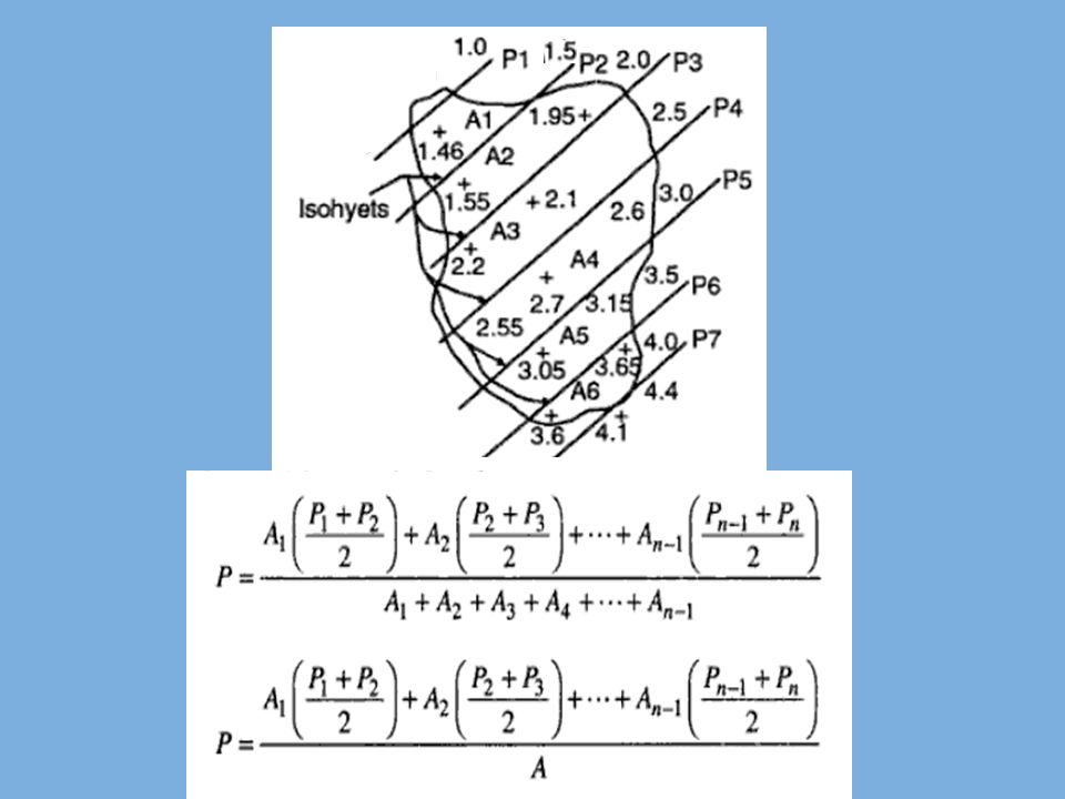
33. Isohyetal Method More accurate than other methods
Location and precipitation are plotted
Contours of equal precipitation called Isohyets are drawn
Calculate area between successive isohyets
The equivalent uniform depth of precipitation between isohyets is assumed to be equal to the median value of two isohyets
This too is an area-based weighting scheme. Contour lines of equal precipitation are estimated from the point measurements.

35. Adjustment for Missing Data
If rain gauge data at 1 or 2 stations is missing
Interpolation in the estimation of average rainfall
Data from neighboring stations is used
‘Normal Rainfall’ used as a standard for comparison
‘Normal Rainfall’ is the average value of rainfall at a particular date, month or year over a specified 30-year period.
Reciprocal Distance Method

36. Estimating Point Rainfall at a given Location
Interpolation
From recorded values at surrounding sites
Arithmetic Mean Method
Inverse distance square
Normal Ratio Method
Station Year Method
Double Mass Curve
Source: Hydrology and Flood Plain Analysis

37. Arithmetic Mean Method
Break in station data
Requires data from at least 3 other stations (evenly distributed) close to that station
Normal precipitation at other stations should be within 10% of precipitation at that station
PA, PB, PC = Precipitation at nearby stations
Px = Estimated precipitation of the missing station
The 3 stations are called index stations.
30 years of data is required to calculate normal annual precipitation.

38. Inverse Distance From recorded values at surrounding sites
Based on weighted average of surrounding values
The weights are reciprocals of the sum of square of distances D, measured from the point of interest
Source: Hydrology and Flood Plain Analysis

39. Normal Ratio Method
When normal annual precipitation of nearby stations ( NA, NB, NC, ..) differs more than 10% of that of the station (Nx) with missing data
N= Normal Precipitation
Normal precipitation = N
Precipitation = P

40. Station Year Method
Record of 2 or more independent stations are combined
Area of these stations should be climatologically same
Missing record at certain station in particular year is found by ratio of the average
PA2000/PA1999 = PB2000/PB1999
Check with another station C and if the two results differ slightly then take average of two results.

41. Double Mass Analysis
For checking the consistency of a station against one or more nearby stations
Consider a station E collecting data for 45 years
For some reasons, the catch of the station is affected
There are other stations H and I with same storm patterns though their annual rainfall differ
Check for a consistent correlation between the averages of H and I and that of E in early years
Plot the accumulated annual rainfall at E against the accumulated average annual rainfall at H and I
Correct the existing rainfall catch at E when the relationship changes against the previous relationship
Annual rainfall of H and I may differ due to elevation differences or some other factors.

42. Double Mass Curve

43. Rain-Gauge Data Spatial Interpolation
When interpolation methods are appropriate?
when an attribute measured at sample points is a spatially continuous field variable
Involves estimating the rainfall values at unmeasured points
The common problem of obtaining rainfall data for the watershed of interest using point rain gauges is addressed using spatial interpolation procedures.

44. Spatial Interpolation Methods
Nearest neighbor (Thiessen Polygon Method )
Isohyetal
Triangulation
Distance weighting
Krigging
The nearest-neighbor method simply assigns a value to the grid equaling the value of the nearest data point.

45. Triangulation
Joining of adjacent data points by a line to form a lattice of triangles (TIN)
Values at any intermediate point on the surface can be computed through trigonometry

46. Distance weighting
Moving-average procedure using points within a specified zone of influence
Example: Inverse distance weighting
weights are inversely proportional to the square of the distance between the point of interest and each of the data points
Powers other than 2 may be used to change the rate of decay of the weighting function.

47. Kriging
Also based on a weighted sum of the points within a zone of influence
weights in kriging are determined from a set of n simultaneous linear equations, where n is the number of points used for the estimation
Based on spatial correlation
points closer together tend to be strongly correlated, whereas those far apart lack correlation
The spatial correlation, expressed as the covariance between pairs of sample points and the sample points being estimated, is first computed and the weights then determined. Over the field of interest, the variogram is formed as an inverse plot of the autocorrelogram, the covariance versus distance. Variograms provide a measure of the spatial continuity of the interpolated surface.

48. PRISM? Parameter-elevation Regressions on Independent Slopes Model
Expert system that uses point data and a digital elevation model (DEM) to generate gridded estimates of climate parameters
Developed to overcome the deficiencies of standard spatial interpolation methods, where orographic effects strongly influence weather patterns
PRISM has been used to map temperature, snowfall, weather generator statistics, and others
Uses DEM

49. PRISM (conti..)
For each DEM grid cell, PRISM develops a weighted precipitation/elevation (P/E) regression function from nearby stations, and predicts precipitation at the cell’s DEM elevation with this function
In the regression, greater weight is given to stations with locations, elevations, and topographic positionings similar to that of the grid cell
Whenever possible, PRISM calculates a prediction interval for the estimate, which is an approximation of the uncertainty involved.
topographic positions (terrain elements, or topographic features)

50. Hyetograph, Mass Curve and Hydrograph
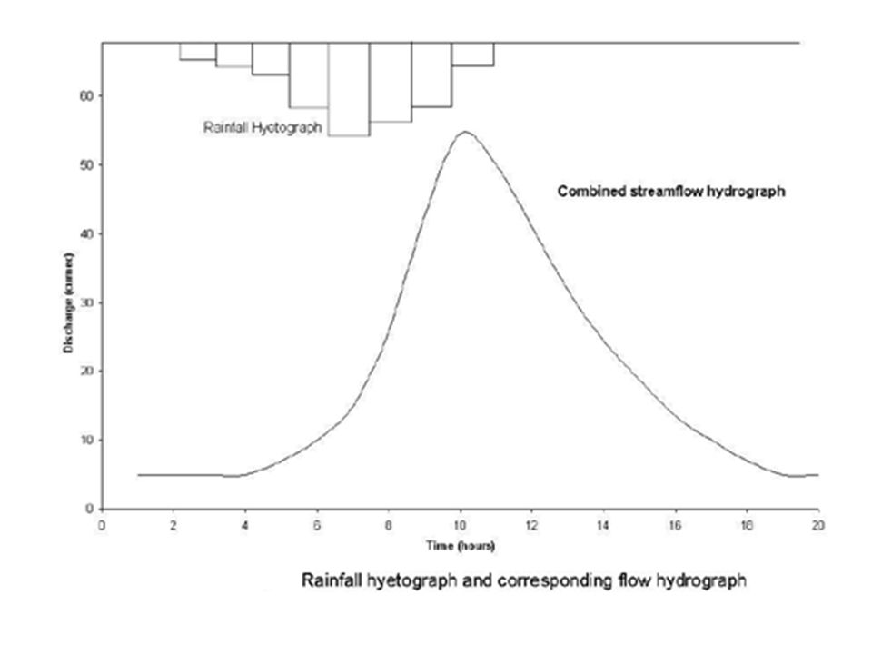
Hyetograph is the graphical plot of the rainfall plotted against time
Mass Curve of rainfall is a plot of accumulated rainfall against time
Hydrograph is a plot of discharge in the channel vs. time (cubic feet per second)
Hydrograph after separating the base flow is called Direct Runoff Hydrograph
Hyetograph: Plot of rainfall intensity (in/hr) verses time
Hydrograph: Time history of rainfall intensity. Plot of flow rate vs. time measured at a stream cross section primarily made up of overland flow.
Hydrologic response of rainfall at the outlet of an area
plot of the stream flow at a particular location as a function of time.
Actual shape and timings of the hydrograph is determined largely by the size, shape, slope, and storage in the basin and by the intensity and duration of input rainfall.

51. Plotting a Hyetograph
Discrete representation of rainfall hydrograph
Source: Das and Saikia
Area under hyetograph represents the total rainfall received in the period

53. Rainfall Mass Curve
Plot of accumulated rainfall against time

54. END

55. Elementary Engineering Hydrology
 By Deodhar M. J.