1. Wflow OpenStreams A short description and selected case studies

2. Hydrological models wflow* Fully distributed Source maps needed: DEM Land-use [can be uniform] Soil [ can be uniform] Preparation script that performs the landscape analysis (catchment delineation etc.) All model parameters linked to land-use/soil maps Can perform state updating in real-time applications Written in python and pcraster Flexible and open Part of the Deltares OpenStreams Initiative (www.openstreams.nl)

3. Doc and source via wflow.googlecode.com

4. Why python/pcraster? Can use (parts of) exiting pcraster modules Can use python for generic programming (command-line options, reading XML, updating, debugger, IDE etc) Free! (as in Speech and Beer) Fast! If you can avoid loops and perform all operation on vectors/matrices Other operations can also be done in python: Retrieving ftp data, link to openDAP Data copying and cleaning Logging Plotting and analysis (similar to Matlab) etc.

5. Why another model? We used existing concepts and put them in a new framework The models available balance between conceptual and physical representation of the catchment New data sets (DEM, RS data etc) cannot be used by many existing models -> this framework should allow that This models maximize the use of available (spatial) data They Can be used in data rich and data sparse environments

6. Currently available wflow_sbm.py – Simple Bucket model (physically based) that includes lateral groundwater flow and used a exponential decay of Ksat with depth wflow_hbv.py – distributed version of the conceptual HBV96 model wflow_W3RA.py – A global hydrological model using two vegetation fractions (CSIRO) wflow_gr4.py – a distributed version of the gr4 model (CEMAGREF) wflow_routing.py – a kinematic wave based routing model (can use input from the hydrological concepts) wflow_wave.py – a dynamic wave model that can be run nexted in the wflow_routing model for the main rivers wflow_floodmap.py – a simple flood mapping routine that can be used a as step after wflow_routing of wflow_wave

7. Scale, grid size Estimated grid size constraints based on the concepts in the model wflow_sbm.py – 5x5m to 4x4km wflow_hbv.py – 500x500m 40x40km wflow_W3RA.py – 10x10km to 0.5x0.5 degree wflow_gr4.py – 500x500m 40x40km wflow_routing.py – 5x5m to 0.5x0.5 degree wflow_wave.py – 5x5m to 1x1km wflow_floodmap.py – 5x5m to 1x1km Clearly, these are very rough estimates, based on actual applications and expert judgemend, YMMV!

8. Applications Typical applications of the models. Theseare estimated and the model are not specifically designed for these application. In addition, the model can also be used for other applications. Process hydrology – wflow_sbm, wflow_W3RA Water resources – wflow_sbm, wflow_W3RA Flow forecasting – wflow_hbv, wflow_gr4, wflow_sbm, wflow_routing, wflow_wave Climate change impact – wflow_sbm, wflow_hbv, wflow_W3RA Land use change impact – wflow_sbm, wflow_W3RA, wflow_hbv

9. Ok What can it do? Simulations of water level and discharge (for simulations or operational purposes) Investigate the effect of a changing environment (climate, land used, e.g. urbanisation) Can work on different catchment sizes All variables are distributed in space Can start simple and expand later on Bandung Rhine

10. 1: Terrain analysis 1.Optional cutout part of DEM 2.Set outlet at lowest gauge and extra points (for later output) at other gauges using gauge coordinates 3.Determine river network (can use existing to burn-in if needed) 4.Determine LDD and sanitized DEM 5.Resample land-use map to DEM

11. 1: Terrain analysis wflow_catchment.map wflow_dem.map wflow_gauges.map wflow_landuse.map wflow_ldd.map wflow_river.map wflow_streamorder.map wflow_subcatch.map …. These maps (the model structure can be used by all models

12. 2: Model parameters All parameters are linked to land- use/soil types via so called lookup tables Links parameters to land-use map and/or soil map Calibration/Verification step

13. Detail wflow_sbm

14. The processes: Interception Rainfall interception via Gash model → daily timesteps

15. The processes: The soil Soil accounting scheme based on TOPOG_SBM (Vertessy and Elsenbeer 1999) Schematic representation of the hydrologic processes modeled by Topog_SBM. Symbol definitions: rf, rainfall; in, infiltration; st, transfer between unsaturated and saturated zone; ie, infiltration excess; se, saturation excess; ex, exfiltration; of, overland flow; and sf, subsurface flow.

16. The processes: The soil Inputs to the model: Et + Es from the canopymodel Total throughfall + stemflow from the canopy model Determines: In- exfiltration Lateral saturated flow Transfer between saturated and unsaturated store Reduces Et + Es to an 'actual evaporation' if water stress occurs (takes rooting depth into account). Surface runoff via kinematic wave -> wflow_routing

17. The processes: The soil Ksat decreases exponentially in depth (M parameter) Transfer between unsaturated and saturated store based on K at that depth Infiltration can include sub-cell parameters for % of compacted soil.

18. Effect of the M parameter

19. Guinea Flow from rivers needed for coastal study Q only for one (small) station No P and ET Setup: DEM and catchment from SRTM Uniform soil, parameters estimated (soil depth from landscape) P from TRRM, ET from re-analysis Run for 10 years to get flows November 30 2011

20. Guinea

21. Rainfall November 30 2011

22. Guinea flow

23. Wflow_sbm for Rhine Description of the model at www.openstreams.nlwww.openstreams.nl In short: HBV Snowmelt Mass wasting of snow Gash rainfall interception Topog_SBM soil Soil temp for frozen soil Kinematic wave November 30 2011

24. Wflow_sbm for Rhine Soil decrease of Ksat with depth Subgrid saturation depending on altitude in a cell November 30 2011

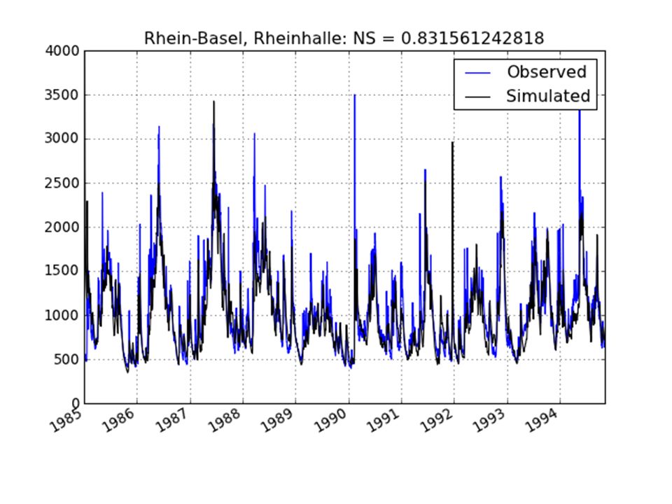
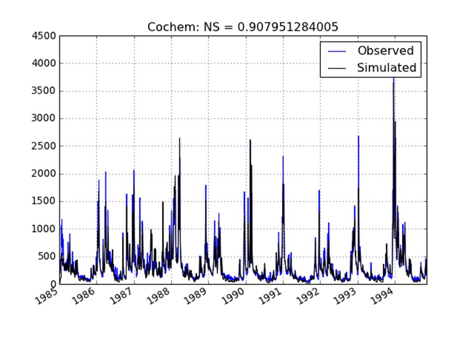
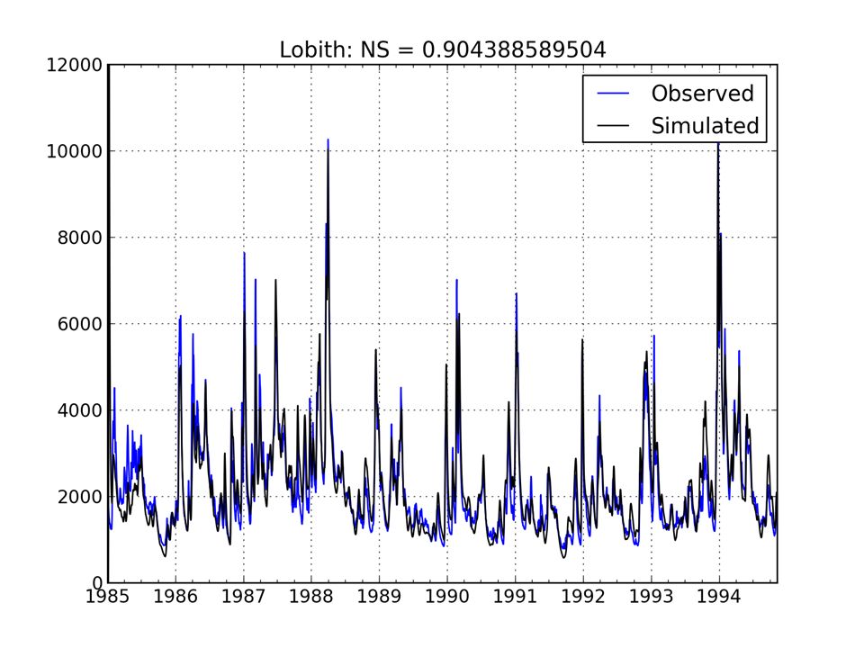
25. Calibration for Rhine: http://schj.home.xs4all.nl/html/calib_report.html EOBS Precip and Temp -> ET derived from EOBS using Hargreaves 1985 – 1995: Rhein-Basel, Rheinhalle Kalkhoven Rockenau Kaub Koeln Lobith Raunheim Cochem Andernach Maxau Schermbeck Menden Hattingen November 30 2011

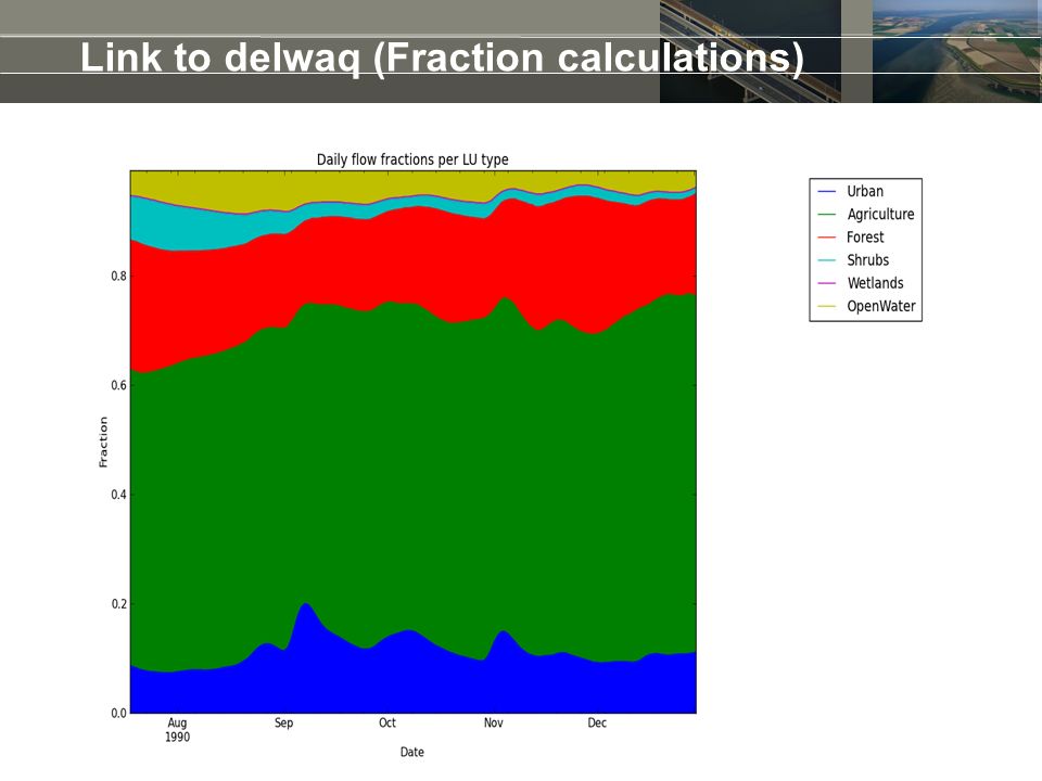
29. Link to delwaq (Fraction calculations)

31. Thanks! For more information: www.openstreams.nl Jaap.schellekens@deltares.nl