2. Fibonacci Numbers, Vector Programs and a new kind of science

3. Sequences That Sum To n Let f n+1 be the number of different sequences of 1’s and 2’s that sum to n. Example: f 5 = 5

4. Sequences That Sum To n Let f n+1 be the number of different sequences of 1’s and 2’s that sum to n. Example: f 5 = 5 4 = 2 + 2 2 + 1 + 1 1 + 2 + 1 1 + 1 + 2 1 + 1 + 1 + 1

5. Sequences That Sum To n f1f1 f2f2 f3f3 Let f n+1 be the number of different sequences of 1’s and 2’s that sum to n.

6. Sequences That Sum To n f 1 = 1 0 = the empty sum f 2 = 1 1 = 1 f 3 = 2 2 = 1 + 1 2 Let f n+1 be the number of different sequences of 1’s and 2’s that sum to n.

7. Sequences That Sum To n f n+1 = f n + f n-1 Let f n+1 be the number of different sequences of 1’s and 2’s that sum to n.

8. Sequences That Sum To n f n+1 = f n + f n-1 Let f n+1 be the number of different sequences of 1’s and 2’s that sum to n. # of sequences beginning with a 2 # of sequences beginning with a 1

9. Leonardo Fibonacci In 1202, Fibonacci proposed a problem about the growth of rabbit populations.

10. Rules 1.in the first month there is just one pair 2.new-born pairs become fertile after their second month 3.each month every fertile pair begets a new pair, and 4.the rabbits never die

11. Inductive Definition or Recurrence Relation for the Fibonacci Numbers Stage 0, Initial Condition, or Base Case: Fib(0) = 0; Fib (1) = 1 Inductive Rule For n>1, Fib(n) = Fib(n-1) + Fib(n-2) n01234567 Fib(n)0112358 1313

12. Fibonacci Numbers Again f n+1 = f n + f n-1 f 1 = 1 f 2 = 1 Let f n+1 be the number of different sequences of 1’s and 2’s that sum to n.

13. Visual Representation: Tiling Let f n+1 be the number of different ways to tile a 1 × n strip with squares and dominoes.

14. Visual Representation: Tiling Let f n+1 be the number of different ways to tile a 1 × n strip with squares and dominoes.

15. Visual Representation: Tiling 1 way to tile a strip of length 0 1 way to tile a strip of length 1: 2 ways to tile a strip of length 2:

16. f n+1 = f n + f n-1 f n+1 is number of ways to tile length n. f n tilings that start with a square. f n-1 tilings that start with a domino.

17. Let’s use this visual representation to prove a couple of Fibonacci identities.

18. Fibonacci Identities Some examples: F 2n = F 1 + F 3 + F 5 + … + F 2n-1 F m+n+1 = F m+1 F n+1 + F m F n (F n ) 2 = F n-1 F n+1 + (-1) n

19. F m+n+1 = F m+1 F n+1 + F m F nmn m-1n-1

20. (F n ) 2 = F n-1 F n+1 + (-1) n

21. n-1 F n tilings of a strip of length n-1

22. (F n ) 2 = F n-1 F n+1 + (-1) nn-1 n-1

23. n (F n ) 2 tilings of two strips of size n-1

24. (F n ) 2 = F n-1 F n+1 + (-1) n n Draw a vertical “fault line” at the rightmost position (<n) possible without cutting any dominoes

25. (F n ) 2 = F n-1 F n+1 + (-1) n n Swap the tails at the fault line to map to a tiling of 2 n-1 ‘s to a tiling of an n-2 and an n.

26. (F n ) 2 = F n-1 F n+1 + (-1) n n Swap the tails at the fault line to map to a tiling of 2 n-1 ‘s to a tiling of an n-2 and an n.

27. (F n ) 2 = F n-1 F n+1 + (-1) n-1 n even n odd

28. The Fibonacci Quarterly

29. Vector Programs Let’s define a (parallel) programming language called VECTOR that operates on possibly infinite vectors of numbers. Each variable V ! can be thought of as: 0 1 2 3 4 5.........

30. Vector Programs Let k stand for a scalar constant will stand for the vector = V ! + T ! means to add the vectors position-wise. + =

31. Vector Programs RIGHT(V ! ) means to shift every number in V ! one position to the right and to place a 0 in position 0. RIGHT( ) =

32. Vector Programs Example: V ! := ; V ! := RIGHT(V ! ) + ; V ! = V ! = Store V ! = V ! = V ! =

33. Vector Programs Example: V ! := ; Loop n times: V ! := V ! + RIGHT(V ! ); V ! = n th row of Pascal’s triangle. Store V ! =

34. X1 X1 X2 X2 + + X3 X3 Vector programs can be implemented by polynomials!

35. Programs -----> Polynomials The vector V ! = will be represented by the polynomial:

36. Formal Power Series The vector V ! = will be represented by the formal power series:

37. V ! = is represented by 0 is represented by k RIGHT(V ! ) is represented by (P V X) V ! + T ! is represented by (P V + P T )

38. Vector Programs Example: V ! := ; Loop n times: V ! := V ! + RIGHT(V ! ); V ! = n th row of Pascal’s triangle. P V := 1; P V := P V + P V X;

39. Vector Programs Example: V ! := ; Loop n times: V ! := V ! + RIGHT(V ! ); V ! = n th row of Pascal’s triangle. P V := 1; P V := P V (1+ X);

40. Vector Programs Example: V ! := ; Loop n times: V ! := V ! + RIGHT(V ! ); V ! = n th row of Pascal’s triangle. P V = (1+ X) n

41. Let’s add an instruction called PREFIXSUM to our VECTOR language. W ! := PREFIXSUM(V ! ) means that the i th position of W contains the sum of all the numbers in V from positions 0 to i.

42. What does this program output? V ! := 1 ! ; Loop k times: V ! := PREFIXSUM(V ! ) ; k’th Avenue 0 1 2 3 4

43. Al Karaji Perfect Squares Zero_Ave := PREFIXSUM( ); First_Ave := PREFIXSUM(Zero_Ave); Second_Ave :=PREFIXSUM(First_Ave); Output:= RIGHT(Second_Ave) + Second_Ave Second_Ave = <1, 3, 6, 10, 15,. RIGHT(Second_Ave) = <0, 1, 3, 6, 10,. Output = <1, 4, 9, 16, 25

44. Can you see how PREFIXSUM can be represented by a familiar polynomial expression?

45. How to divide polynomials? 1 1 – X ? 1 1 -(1 – X) X + X -(X – X 2 ) X2X2 + X 2 -(X 2 – X 3 ) X3X3 = 1 + X + X 2 + X 3 + X 4 + X 5 + X 6 + X 7 + … …

46. 1 + X 1 + X 2 + X 3 + … + X n + ….. = 1 + X 1 + X 2 + X 3 + … + X n + ….. = 1 1 - X The Infinite Geometric Series

47. W ! := PREFIXSUM(V ! ) is represented by P W = P V / (1-X) = P V ( 1+X+X 2 +X 3 + ….. )

48. Al-Karaji Program Zero_Ave = 1/(1-X); First_Ave = 1/(1-X) 2 ; Second_Ave = 1/(1-X) 3 ; Output = 1/(1-X) 3 + X/(1-X) 3 = (1+X)/(1-X) 3

49. (1+X)/(1-X) 3 Zero_Ave := PREFIXSUM( ); First_Ave := PREFIXSUM(Zero_Ave); Second_Ave :=PREFIXSUM(First_Ave); Output:= RIGHT(Second_Ave) + Second_Ave Second_Ave = <1, 3, 6, 10, 15,. RIGHT(Second_Ave) = <0, 1, 3, 6, 10,. Output = <1, 4, 9, 16, 25

50. (1+X)/(1-X) 3 outputs outputs X(1+X)/(1-X) 3 outputs outputs The k th entry is k 2 The k th entry is k 2

51. X(1+X)/(1-X) 3 =  k 2 X k What does X(1+X)/(1-X) 4 do?

52. X(1+X)/(1-X) 4 expands to :  S k X k where S k is the sum of the first k squares

53. Aha! Thus, if there is an alternative interpretation of the k th coefficient of X(1+X)/(1-X) 4 we would have a new way to get a formula for the sum of the first k squares.

54. What is the coefficient of X k in the expansion of: ( 1 + X + X 2 + X 3 + X 4 +.... ) n ? Each path in the choice tree for the cross terms has n choices of exponent e 1, e 2,..., e n ¸ 0. Each exponent can be any natural number. Coefficient of X k is the number of non-negative solutions to: e 1 + e 2 +... + e n = k

55. What is the coefficient of X k in the expansion of: ( 1 + X + X 2 + X 3 + X 4 +.... ) n ?

56. ( 1 + X + X 2 + X 3 + X 4 +.... ) n =

57. Using pirates and gold we found that: THUS:

58. Vector programs -> Polynomials -> Closed form expression

59. A big jump Let’s jump into the world of simple programs

60. Cellular automata

62. The main discovery A simple program can create complex output

63. 4 kinds of behavior

64. Why these discoveries were not made before? New technologies!

65. A hypothesis Cellular automata are an exception!

66. Other simple programs

67. 3 colors

68. Being mobile Not parallel!

69. Mobile Automata

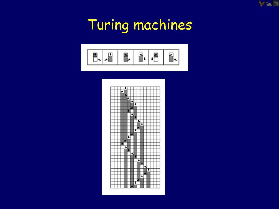
71. Turing machines

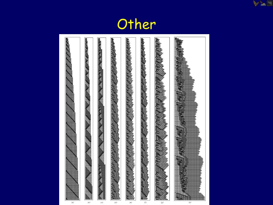
73. Other

74. First conclusions Phenomena of Complexity can be found in a variety of simple programs!

75. Systems based on Numbers

76. But…

78. A hypothesis This is all because of the representation in base 2!

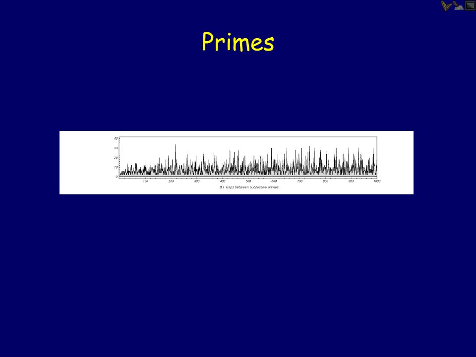
80. Primes

81. Pi

82. Functions

84. Conclusion Other systems can exhibit the same behavior as cellular automatas

85. Chaos phenomena

86. Start with 1/2

87. Start with random value

88. Tiny perturbations of the input

89. Can (d) create randomness? No! Random input can lead to random output But (a) and (b) can!

90. Continuous

91. Conclusion Same results in continuous and discrete First discovered in discrete because easier to investigate Continuous is like average of discrete

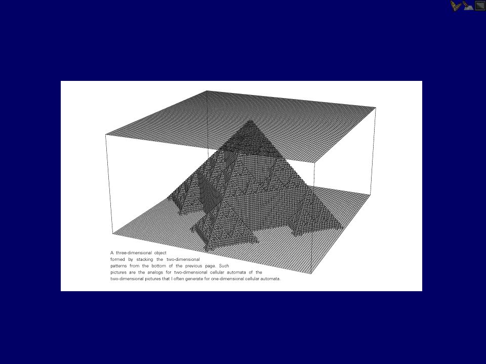
92. Dimensions

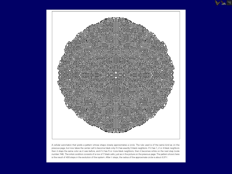
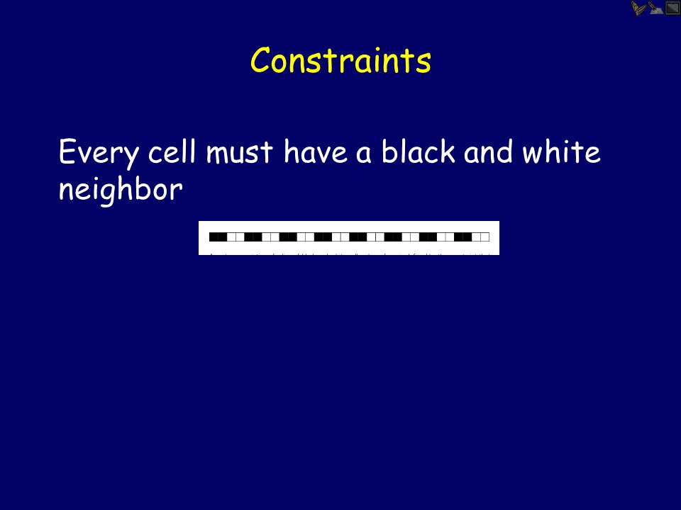
96. Constraints Every cell must have a black and white neighbor

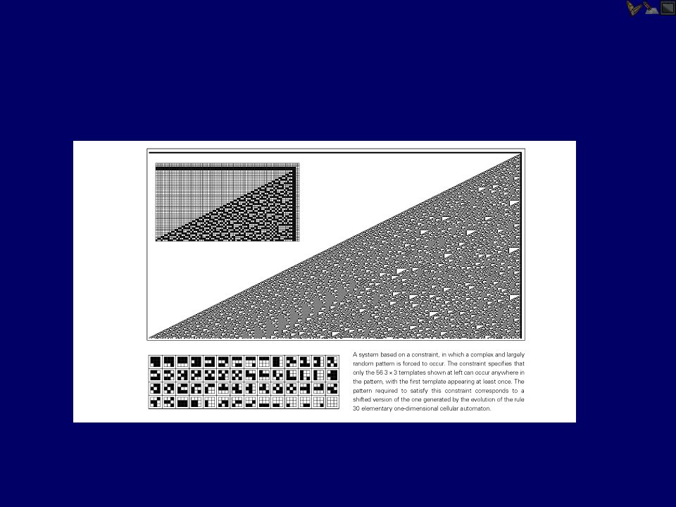
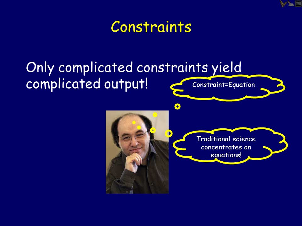
99. Constraints Only complicated constraints yield complicated output! Constraint=Equation Traditional science concentrates on equations!

100. A hypothesis Starting from randomness no order can emerge

102. Conclusion Order can emerge from randomness

103. Four classes of behavior

104. Sources of randomness New!

105. Is this useful?

106. Snow flakes

107. Growth of plants

108. Computation

109. Is there a universal cellular automata? Yes!

111. Take home message Thinking in terms of programs instead of equations can lead to new insights A simple program could produce all the complexity we see.

112. …Go and find it!

113. REFERENCES Coxeter, H. S. M. ``The Golden Section, Phyllotaxis, and Wythoff's Game.'' Scripta Mathematica 19, 135-143, 1953. "Recounting Fibonacci and Lucas Identities" by Arthur T. Benjamin and Jennifer J. Quinn, College Mathematics Journal, Vol. 30(5): 359--366, 1999. Stephen Wolfram, “A New Kind of Science”, 2002