Download presentation
Presentation is loading. Please wait.

1
National Center for Supercomputing Applications University of Illinois at Urbana-Champaign Variant Calling Workshop

2
Overview There will be two parts to the workshop: Variant calling analysis (on the cluster) Visualization (on the desktop) using IGV Command prompts (what you will type) will be in boxes preceded by ‘$’. Output will be in red: $ mkdir foo $ cd foo $ ls -la total 96 drwxrwxr-x 2 cjfields cjfields 32768 Jun 23 22:51. drwxr-x--- 39 cjfields cjfields 32768 Jun 23 22:51..

3
Prelude : Variant Calling Setup 1.Log into the cluster using your classroom account. 2.Create a work folder (I call mine ‘mayo_test’): $ mkdir mayo_test $ cd mayo_test $ ll total 0
: $ mkdir mayo_test $ cd mayo_test $ ll total 0.")
4
Part Ia : Variant Calling Setup 3.Link in all scripts from the main work folder to this directory: $ ln -s /home/mirrors/gatk_bundle/mayo_workshop/*.sh. $ ls annotate_snpeff.sh call_variants_ug.sh hard_filtering.sh post_annotate.sh

5
Data for this workshop is from the 1000 Genomes project and is WGS, 60x coverage The initial part of the GATK pipeline (alignment, local realignment, base quality score recalibration) has been done, and the BAM file has been reduced for a portion of human chromosome 20 Otherwise, we would not even finish the alignment within the next few days, let alone the other steps Part Ia : Variant Calling Setup
 has been done, and the BAM file has been reduced for a portion of human chromosome 20 Otherwise, we would not even finish the alignment within the next few days, let alone the other steps Part Ia : Variant Calling Setup")
6
Part Ia : Variant Calling Start the variant calling job. Check the status of the job using ‘qstat’: $ qsub call_variants_ug.sh 371875.biocluster.igb.illinois.edu $ qstat -u biocluster.igb.illinois.edu: Req'd Req'd Elap Job ID Username Queue Jobname SessID NDS TSK Memory Time S Time -------------------- ----------- -------- ---------------- ------ ----- ------ ------ ----- - ----- 371875.biocluste cjfields default call_variants_ug 24285 1 4 10gb -- R 00:01

7
Part Ia : Variant Calling Discussion: what did we just do? We ran the GATK UnifiedGenotyper to call variants Show the script…

8
Part Ia : Variant Calling Job done yet? Should only be a few minutes… What do the data look like? (anyone here use UNIX?) $ qstat -u $ ll *vcf* -rw-rw-r-- 1 cjfields cjfields 237060 Jun 23 23:10 raw_indels.vcf -rw-rw-r-- 1 cjfields cjfields 2829 Jun 23 23:10 raw_indels.vcf.idx -rw-rw-r-- 1 cjfields cjfields 3203447 Jun 23 23:08 raw_snps.vcf -rw-rw-r-- 1 cjfields cjfields 107241 Jun 23 23:08 raw_snps.vcf.idx $ tail -n 2 raw_indels.vcf 2026306897rs200138621CAGAC1305.73. AC=1;AF=0.500;AN=2;BaseQRankSum=3.130;DB;DP=75;FS=0.936;MLEAC=1;MLEAF=0.500;MQ=57.75;MQ0=0;MQRan kSum=0.407;QD=5.80;ReadPosRankSum=0.371GT:AD:DP:GQ:PL0/1:44,26:75:99:1343,0,2526 2026314306rs199619140GTG1502.73. AC=1;AF=0.500;AN=2;BaseQRankSum=3.814;DB;DP=83;FS=0.000;MLEAC=1;MLEAF=0.500;MQ=57.12;MQ0=0;MQRan kSum=-1.411;QD=18.11;ReadPosRankSum=1.387GT:AD:DP:GQ:PL0/1:33,36:76:99:1540,0,1253
 $ qstat -u $ ll *vcf* -rw-rw-r-- 1 cjfields cjfields Jun 23 23:10 raw_indels.vcf -rw-rw-r-- 1 cjfields cjfields 2829 Jun 23 23:10 raw_indels.vcf.idx -rw-rw-r-- 1 cjfields cjfields Jun 23 23:08 raw_snps.vcf -rw-rw-r-- 1 cjfields cjfields Jun 23 23:08 raw_snps.vcf.idx $ tail -n 2 raw_indels.vcf rs CAGAC AC=1;AF=0.500;AN=2;BaseQRankSum=3.130;DB;DP=75;FS=0.936;MLEAC=1;MLEAF=0.500;MQ=57.75;MQ0=0;MQRan kSum=0.407;QD=5.80;ReadPosRankSum=0.371GT:AD:DP:GQ:PL0/1:44,26:75:99:1343,0, rs GTG AC=1;AF=0.500;AN=2;BaseQRankSum=3.814;DB;DP=83;FS=0.000;MLEAC=1;MLEAF=0.500;MQ=57.12;MQ0=0;MQRan kSum=-1.411;QD=18.11;ReadPosRankSum=1.387GT:AD:DP:GQ:PL0/1:33,36:76:99:1540,0,1253.")
9
Part Ia : Variant Calling How many SNPs and Indels were called? Any found in dbSNP? $ grep -c -v '^#' raw_snps.vcf 13621 $ grep -c -v '^#' raw_indels.vcf 1070 $ grep -c 'rs[0-9]*' raw_snps.vcf 12245 $ grep -c 'rs[0-9]*' raw_indels.vcf 1019

10
Part Ib : Hard filtering We need to filter the variant calls Generally, for human data we would use variant quality score recalibration, but we have a very small set of variants, so here we use hard filtering

11
Part Ib : Hard filtering Start the hard filtering step. This will be fast: You will have two new VCF files in a minute: hard_filtered_snps.vcf hard_filtered_indels.vcf $ qsub hard_filtering.sh 371886.biocluster.igb.illinois.edu $ qstat -u biocluster.igb.illinois.edu: Req'd Req'd Elap Job ID Username Queue Jobname SessID NDS TSK Memory Time S Time -------------------- ----------- -------- ---------------- ------ ----- ------ ------ ----- - ----- 371886.biocluste cjfields default hard_filtering.s 24455 1 4 10gb -- R --

12
Part Ib : Hard filtering What are we doing? Questions: Did we lose any variants? How many PASS’ed the filter? What is the difference in the filtered and raw output?

13
Part Ib : Hard filtering What are we doing? Questions: Did we lose any variants? How many PASS’ed the filter? What is the difference in the filtered and raw output? $ grep -c 'PASS' hard_filtered_snps.vcf 8270 $ grep -c 'PASS' hard_filtered_indels.vcf 1041

14
Part Ic : Annotate the variants (SnpEff) Run the next job, which uses SnpEff to add annotation to the VCF: This takes a couple of minutes… Two new VCF: hard_filtered_snps_annotated.vcf hard_filtered_indels_annotated.vcf $ qsub annotate_snpeff.sh 371894.biocluster.igb.illinois.edu $ qstat -u biocluster.igb.illinois.edu: Req'd Req'd Elap Job ID Username Queue Jobname SessID NDS TSK Memory Time S Time -------------------- ----------- -------- ---------------- ------ ----- ------ ------ ----- - ----- 371894.biocluste cjfields default annotate_snpeff. 18957 1 1 10gb -- R --

15
Part Ic : Annotate the variants (SnpEff) SnpEff adds information about where the variants are in relation to specific genes The IDs for the human assembly version we use are from Ensembl (ENSGXXXXXXXXXXX) The Ensembl ID for FOXA2 is ENSG00000125798
 SnpEff adds information about where the variants are in relation to specific genes The IDs for the human assembly version we use are from Ensembl (ENSGXXXXXXXXXXX) The Ensembl ID for FOXA2 is ENSG")
16
Part Ic : Annotate the variants (SnpEff) The Ensembl ID for FOXA2 is ENSG00000125798 Are there any variants called for FOXA2?
 The Ensembl ID for FOXA2 is ENSG Are there any variants called for FOXA2")
17
Part Ic : Annotate the variants (SnpEff) The Ensembl ID for FOXA2 is ENSG00000125798 Are there any variants called for FOXA2? SnpEff also creates some additional output files; we’ll see those in a bit $ grep -c 'ENSG00000125798' hard_filtered_snps_annotated.vcf 3 $ grep -c 'ENSG00000125798' hard_filtered_indels_annotated.vcf 0

18
Part Id : GATK VariantAnnotator SnpEff adds a lot of information to the VCF. GATK VariantAnnotator helps remove a lot of the extraneous information

19
Part Id : GATK VariantAnnotator The last step: This may take about 5-10 minutes $ qsub post_annotate.sh 371905.biocluster.igb.illinois.edu $ qstat -u biocluster.igb.illinois.edu: Req'd Req'd Elap Job ID Username Queue Jobname SessID NDS TSK Memory Time S Time -------------------- ----------- -------- ---------------- ------ ----- ------ ------ ----- - ----- 371905.biocluste cjfields default post_annotate.sh 24650 1 4 10gb -- R 00:01

20
While this is going on… Let’s start a little tutorial on the Integrated Genome Viewer (also from Broad)
")
21
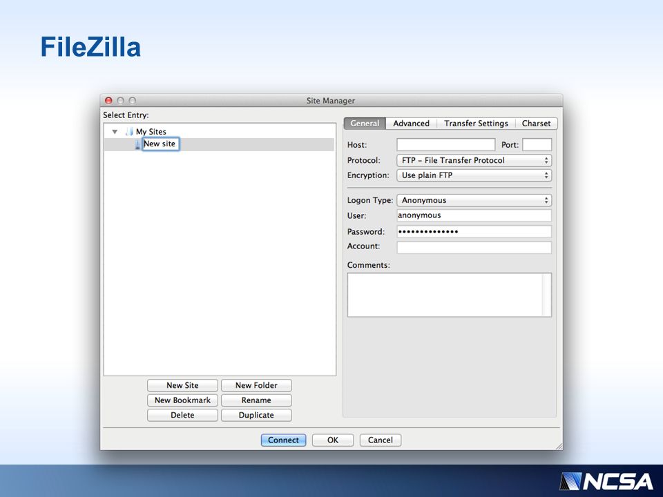
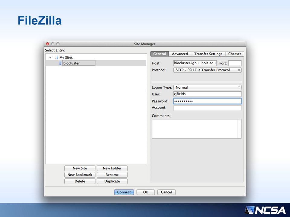
Prelude to Part II We need to download the results from your user folders to the local desktop We’ll use FileZilla for this

22
FileZilla

27
Transfer folder to the desktop

28
Part II : Viewing Results in IGV Open IGV Switch genome to ‘Human (b37)’
’")
29
Part II : Viewing Results in IGV Load the VCF files marked ‘final’ Click on the ‘20’ (chr 20)
")
30
Part II : Viewing Results in IGV Click and drag from the ‘20 mb’ mark to roughly the centromeric region on the chromosome (~2.6 mb)
")
31
Part II : Viewing Results in IGV Click and drag from the ‘20 mb’ mark to roughly the centromeric region on the chromosome (~2.6 mb)
")
32
Part II : Viewing Results in IGV Should look something like this:

33
Part II : Viewing Results in IGV Right click on the track to bring up a menu, and then select ‘Set Feature Visibility Window’ Set to ‘10000000’ (10 million, or 10 mb)
")
34
Part II : Viewing Results in IGV In the search box, enter in ‘FOXA2’ Browser jumps to that gene

35
Part II : Viewing Results in IGV How many SNPs are here? How many indels? How many SNPs are ‘hets’?

36
Part II : Viewing Results in IGV Now we’ll load in a ‘small’ BAM file. This is the same BAM file you analyzed on the cluster In the ‘gatk_bundle’ folder there is a BAM file named ‘ NA12878.HiSeq.WGS.bwa. cleaned.recal.b37.20_arm1. bam ’. Load that file. What is happening here?

37
Part II : Viewing Results in IGV Right click on BAM track and select ‘Show coverage track’ Note colors in coverage track

38
Part II : Viewing Results in IGV Right click on BAM track and select ‘Show coverage track’ Note colors in coverage track

39
Part II : Viewing Results in IGV Zoom in to regions with SNPs Mouse-over the SNP regions in the VCF tracks to get more information (including annotation from SnpEff and VariantAnnotator)
")
40
Browse around… How are filtered SNPs are displayed? How about low-quality bases? Can you change the display to… Sort BAM reads by strand?

41
Part III : SnpEff Results SnpEff gives a nice summary HTML file that should have been downloaded with your result (one for SNP, one for indel results) Open those up in a browser.
 Open those up in a browser.")
42
Part II : Viewing Results in IGV This gives us raw reads, but we need to calculate coverage. Let’s use igvtools. Set command to ‘Count’, then select input file (BAM file). Hit ‘Run’
. Hit ‘Run’.")
Similar presentations