1. CHAPTER 3 NUMERICAL METHODS
Roots of Nonlinear equations
Interpolation (In 2-Dimension)
Numerical Integration
Numerical Solution of Differential Equations

2. 3.1 Roots of Nonlinear Equations
Let say we want to find the solution of f (x) = 0. For example:
These equations can not be solved directly.
We need numerical methods to compute the approximate solutions.

3. Iteration Methods
Let x0 be an initial value that is close to the solution of f (x) = 0. From f (x) = 0, another equation is produced such that we can use x0 to compute x1.
This step is repeated to obtain values of x2, x3,...This method is called Iteration Method.
We hope that every new xi converges to the solution of f (x) = 0.

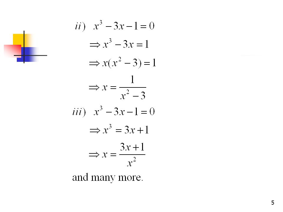
4. Fixed Point Iteration
First we write f (x) = 0 in the form x = F (x).
Note that F (x) is not unique. For instance,
see the following.
Example 3.1

6. We shall use these forms (x = F (x)) in our next example, denoted by

7. For example, see the following figure:
We can say that the solution of x = F (x) is the intersection of two graphs y = x and y = F (x).
For example, see the following figure: y x x0 x1 x2 x3
y0 = x1
y1 = x2
y2 = x3
Figure 3.1 Fixed Point Iteration

8. Solution steps Start the computation with initial value x0.
From y = F (x), we have y0 = F (x0).
Then, from graph y = x, we may assume x1 = y0. From here, we have y1 = F(x1) and x2 = y1.
Similarly, we will obtain x3, x4, … and so on.

9. We hope that the neighborhood denoted by the dashed line converges to the intersection point of the two graphs y = x and y = F(x).
Conclusion
Fixed point iteration is of the form

10. Example 3.2
Approximation by Fixed Point Iteration
(Based on Example 3.1)
In Example 3.1, we have obtained various forms of x = F(x). Now referring to xi+1 = F(xi), we put subscripts as follows.

11. The distance between xi+1 and xi increases,
i.e. |xi+1 – xi| > |xi – xi-1|.
This iteration fails (since it diverges).

12. The distance between xi+1 and xi decreases,
i.e. |xi+1 – xi | < | xi – xi-1 |.
This iteration converges (succeeds).

13. We have |xi+1 – xi | > | xi – xi-1 |
We have |xi+1 – xi | > | xi – xi-1 |. This shows that this iteration diverges (Iteration fails).

14. REMARK
An iteration converges if it satisfies
From the convergent iteration, we conclude that one of the solutions of
CHECK :

15. How to make sure that initial value x0 can give a convergent iteration?
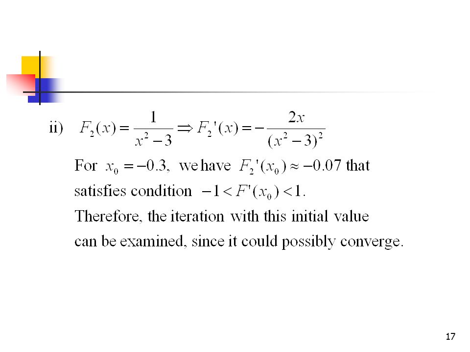
Answer:
We differentiate F(x) to get F ′(x).
The iteration converges if

16. Example 3.3

18. Conclusion

19. 3.1.3 Newton-Raphson Method
Tangent line of f (x) is f ′(x). This is the basic of Newton-Raphson Method described below.
f (x) x
x0 x x2 O
f (x0)
f (x1)
f (x2)
Figure 3.2 Newton-Raphson Method

20. Gradient of the tangent line of f (x) at (x0, f (x0)) is given by f ′(x0). If we continue the tangent line at (x0, f (x0)) to (x1,0), then the gradient of this tangent line can be determined by
Equalizing these two values, we have

21. This means that from the initial value x0, using formula (4), we can compute x1 which is close to the solution of f (x) = 0.
Using the same formula, we can compute x2 which is a better approximation to the solution compare to x1.
We can also compute x3 , x4 , … and so on.
We hope that our iteration converges to the solution of f (x) = 0.

22. In general, Newton-Raphson method can be formulated as

23. Example 3.4 Solution i xi f (xi) f ′ (xi) -1 -3 1 -0.333333 -0.037037-1 -3 1 2 3 -

24. From the table we conclude that:
* xi converges to the solution of f (x) = 0, that is
x 
* Values in column f (xi) go to zero.
(Remark: this shows that we have done a
good approximation)

25. i xi
f (xi)
f ′(xi)
0.99 1 -

26. IMPORTANT!!!
Newton-Raphson method fails if the approximate root of equation, for instance x = x0, close to roots of f ′(x) = 0.
Therefore, we have to make sure that the starting point x0 does not give f ′(x0) close to zero.
The reason is that dividing a number by a value close to zero will give a number with large absolute value.

27. Secant Method
This method is a revision of Newton-Raphson method as described in the following figure.
f (x) x
x0 x1 x2 x3 O
f (x0)
f (x1)
f (x2)
f (x3)
Figure 3.3 Secant Method

28. In this method, we begin with two initial values x0 and x1
In this method, we begin with two initial values x0 and x1. The straight line from (x0, f (x0)) to (x1,f (x1)) is continued to the x-axis.
Let x2 be the value where this straight line intersects the x-axis.
By equalizing gradient from (x0, f (x0)) to (x1, f (x1)) and gradient from (x1, f (x1)) to (x2,0), we obtain

29. Using the same formula, we compute x3, x4, ... and so on.
We hope that xi converges to the solution of f (x) = 0.

30. In general, Secant method can be formulated as

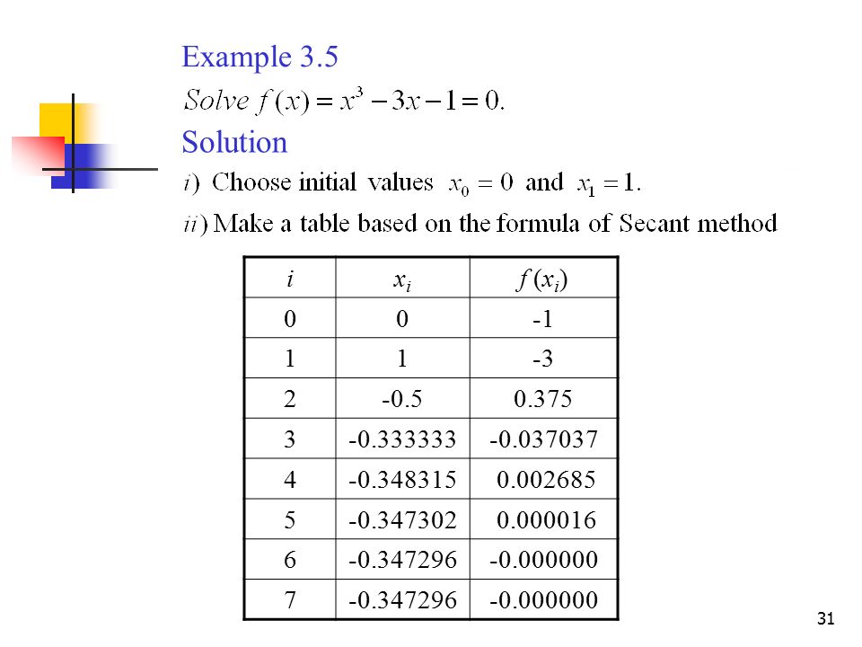
31. Solution Example 3.5 i xi f (xi) -1 1 -3 2 -0.5 0.375 3 -0.333333-1 1 -3 2
-0.5
0.375 3 4 5 6 7

32. From the table, notice that:
* Iteration xi converges to x 
* Values in column f (xi) go to zero.
(Remark as in Newton-Raphson method)
If f (xi) is farer from zero than f (xi -1), then the iteration fails. This means that we made a mistake in estimating xi using this iteration.

33. 3.1.5 How to choose initial values?
Besides conditions of the method we use, we may also see sign of f (x) for the tested x.
For instance, see values of f (x) = x3 – 3x – 1 used in our previous example.
We can make the following sign table:

34. x
f (x)
Sign f (x)
Remark -5
-111
-ve
The sign changes -4
-53 -2 -3
-ve * -1 1
+ve * 2

35. From the sign table, we know that the solution of f (x) = 0 is clearly in between
x = and x = -1,
x = and x = 0,
and x = and x = 2.
If we use Secant Method, we may choose the following
x0 = and x1 = -1,
or x0 = and x1 = 0,
or x0 = and x1 = 2.

36. If we use Fixed Point Method, we can choose x0 that satisfies
If we use Newton-Raphson Method, we focus on the first derivative of f (x) = x3 – 3x – 1,
i.e. f ′(x0) = 3x2 – 3.
We may not choose x0 = -1 or x0 = 1, since this gives f ′(x0) = 0.
But, from the sign table, we may choose x0 = -2 or x0 = 0 or x0 = 2 as long as f ′(x0) is not too close to zero.
If we use Fixed Point Method, we can choose x0 that satisfies

37. 3.2 Interpolation (In 2-dimension)
The meaning of interpolation in 2-dimension is to define a curve that passes through given data points. As an example, see the following: x
Figure Points interpolation

38. 3.2.1 Interpolation Polynomial

39. Example 3.6
Given the data points (0,2), (1,3) and (3,3), what is the unique polynomial that passes through the data points?
Solution
Since we are given three different points, then we can only find unique value for three coefficients: C0, C1 and C2. Then, our interpolation polynomial is quadratic:
y = C0 + C1x + C2x2.

40. If we substitute the given data points (0,2), (1,3) and (3,3) to the polynomial, we get the following three equations:
2 = C0
3 = C0 + C1 + C2
3 = C0 + 3C1 + 9C2.
This is a system of linear equations. The solution is

41. Thus, the unique interpolation polynomial that passes through the given data points is

42. Theorem 3.1 (Interpolation polynomial)

43. There are many methods to find this unique interpolation polynomial
There are many methods to find this unique interpolation polynomial. In this part, we only consider two methods: Lagrange Method and Newton’s Divided Difference Interpolation.

44. Lagrange Method

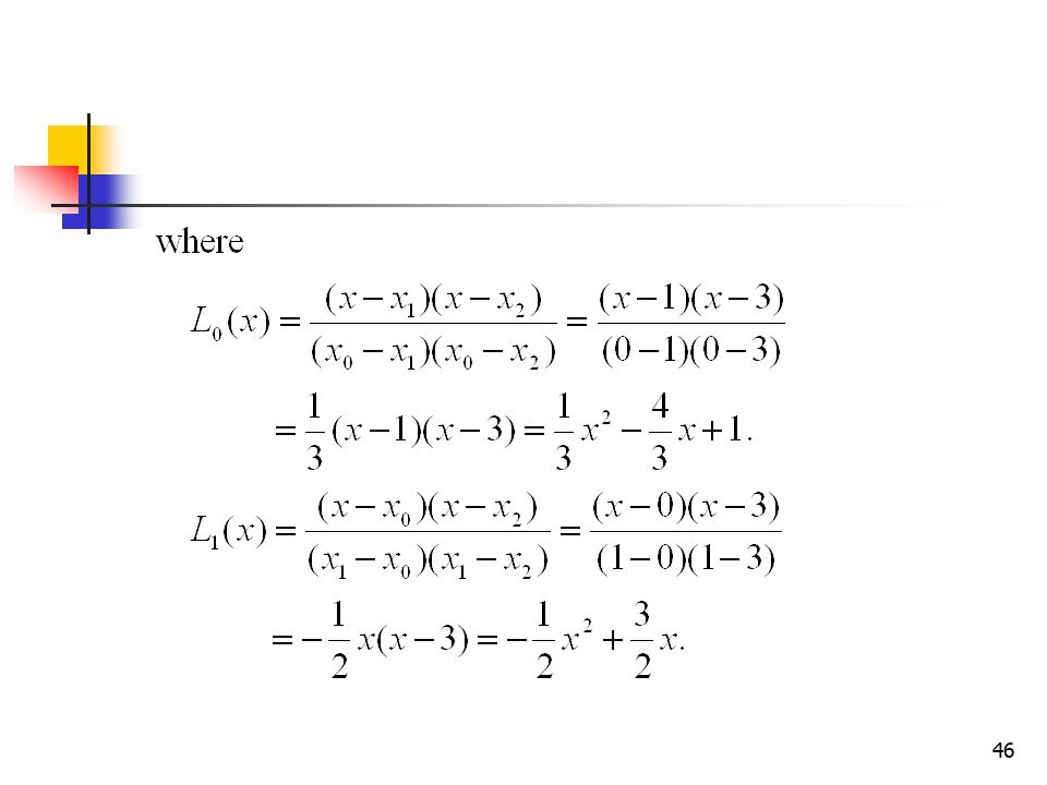
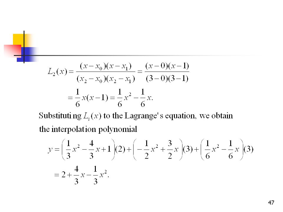
45. Example 3.7
Given the data points (0,2), (1,3) and (3,3). Apply Lagrange Method to find interpolation polynomial passing through these points.
Solution

48. 3.2.3 Newton’s Divided Difference Interpolation
Lagrange method has the following weaknesses:
Lagrange Interpolation Polynomial is hard to find if we have many data points.
If we want to add data, we have to restart our computation from the beginning.
In this part, we discuss a method that can handle the weaknesses of Lagrange Method, called Newton’s Divided Difference Interpolation. Before that, we first need to produce a table of divided difference.

49. 3.2.3.1 Table of Divided Difference

50. Table 3.5 Orders of Divided Difference
Symbol
Definition
f [xi]
f (xi) 1
f [xi , xi +1] 2
f [xi , xi +1 , xi +2] 3
f [xi , xi +1 , xi +2 , xi +3] n
f [x0 , x1 ,…, xn - 1 , xn]

51. Table 3.6 Divided Difference Formulax
f (x) x0
f (x0) x1
f (x1) x2
f (x2) x3
f (x3)

52. Based on Table 3.5, we can produce table of divided difference as in Table 3.6.
Though Table 3.6 shows an estimation for four data points, a similar way can be used for different number of data points.
Example 3.8
Produce a table of divided difference for the following data points:
(1,3), (2,0), (4,8), (3,-8) and (-2,17).
Solution
Table of divided difference for this data is

53. x
f (x) 1 3 2
7/3 4
29/6 8 12
65/72 16
17/8 -8
21/6 -5 -2 17

54. 3.2.3.2 Newton’s Divided Difference Interpolation

55. Example 3.9
Find interpolation polynomial that passes through (0,2), (1,3) dan (3,3) using Newton’s divided difference interpolation.
Solution
Table of divide difference for these three points is x y 2 1 3

57. REMARKS

58. 3.3 Integral Solution Using Numerical Methods
In this part, we discuss the following numerical integration methods:
1) Rectangular Rule
2) Trapezoidal Rule
3) Simpson’s Rule
Before doing the approximation, we first have to give the number of subintervals that we want to consider and find the length of each subinterval.

59. 3.3.1 Number of subintervals and the length of each subinterval
We suppose that the interval from x = a to x = b is divided into n number of subintervals, where the length of each subinterval is
If x0 = a and xn = b, then in general, xi = a + ih.

60. The positions of x0, x1, … ,xn are shown in the following figure.y
| | | | | |
x0 x1 x2 x3  xn
h h
Figure 3.5 Number of subintervals

61. Rectangular Rule
In this method, we suppose that every subinterval forms a rectangle, where the height of each subinterval is
Areas of all rectangles are computed.
Total area of these rectangles is the approximate area below the curve of the function, which is also the estimation of the integral that we want to determine.

62. Figure 3.6 Rectangular Rule
f (x) x y
| | |
x1* x2* x3*
Figure 3.6 Rectangular Rule

63. We have given the length of each subinterval denoted by h.
If the height of the ith rectangle is
then the area of the ith rectangle is
Total area of all rectangles

64. RECTANGULAR RULE

65. Example 3.10
Solution

66. i xi
xi*
f (xi* ) - 1
0.1
0.05 2
0.2
0.15 3
0.3
0.25 4
0.4
0.35 5
0.5
0.45 6
0.6
0.55 7
0.7
0.65 8
0.8
0.75 9
0.9
0.85 10
0.95
TOTAL

67. 3.3.3 Trapezoidal Rule A revision of the Rectangular Rule.
While in the Rectangular Rule we make a rectangle for each subinterval, in Trapezoidal Rule we make a trapezoid for each subinterval.
Areas of all trapezoids are computed.
Total area of all trapezoids is the estimation of the area below the curve of the function, which is also the approximation of the integral of the function.

68. Figure 3.7 Trapezoidal Rule
f (x) x y
x0 x1 x  xn
Figure 3.7 Trapezoidal Rule

69. Thus,
If the length of each subinterval is h,
Height of the left hand side of the ith trapezoid =
Height of the right hand side of the ith trapezoid =
Then the area of the ith trapezoid is

70. Total area of all trapezoids

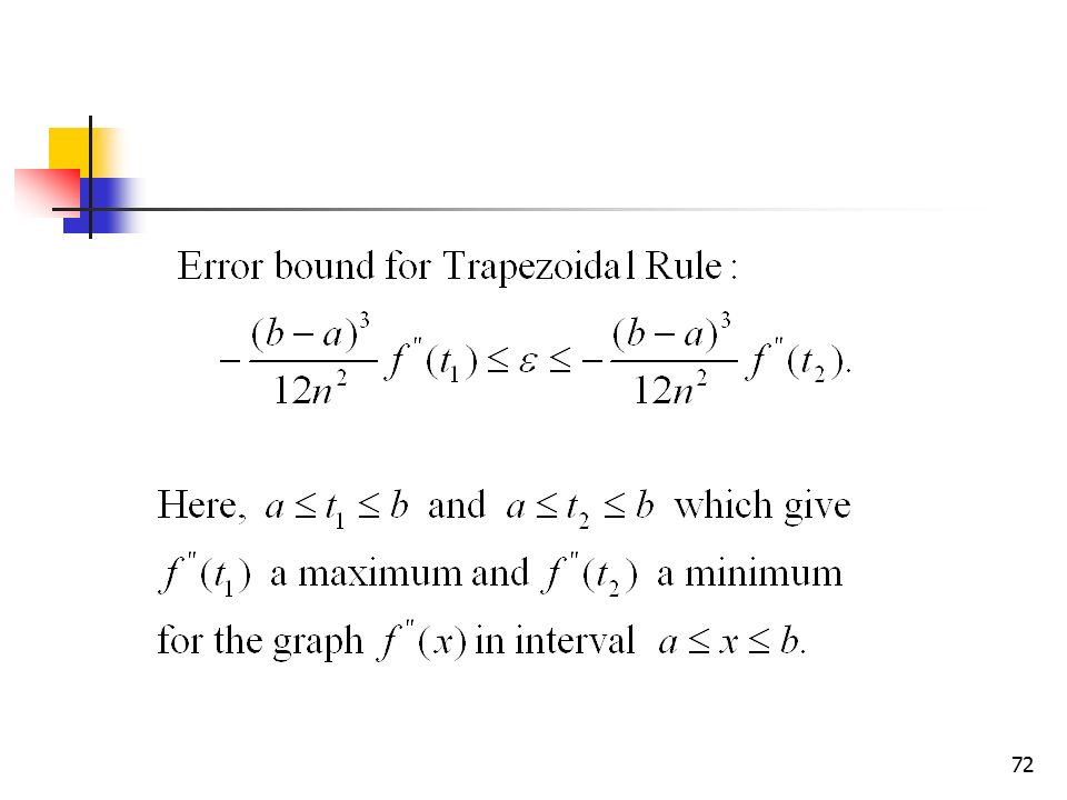
71. TRAPEZOIDAL RULE
where x0 = a and xn = b

73. Example 3.11
Solution

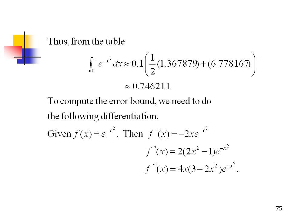
74. i xi
f (a) & f (b )
f (xi ), i=1,…, n-1 1
0.1 2
0.2 3
0.3 4
0.4 5
0.5 6
0.6 7
0.7 8
0.8 9
0.9 10
TOTAL

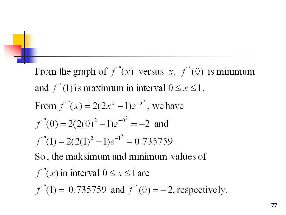
76. Figure 3.7 Trapezoidal Rulex
f (x) O
Figure 3.7 Trapezoidal Rule

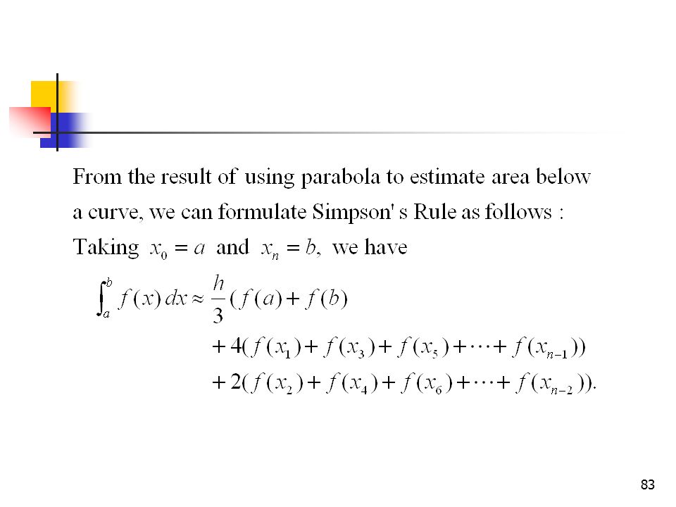
80. Simpson’s Rule
Basic of Rectangular Rule  Using constant to estimate the area of each subinterval.
Basic of Trapezoidal Rule  Using linear equation to estimate the area of each subinterval.
Basic of Simpson’s Rule  Using quadratic equation to estimate the area of each subinterval.

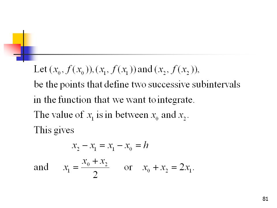
82. x y
x0 x1 x2
h h
P(x) = ax2 + bx + c
Figure 3.7 Simpson’s Rule

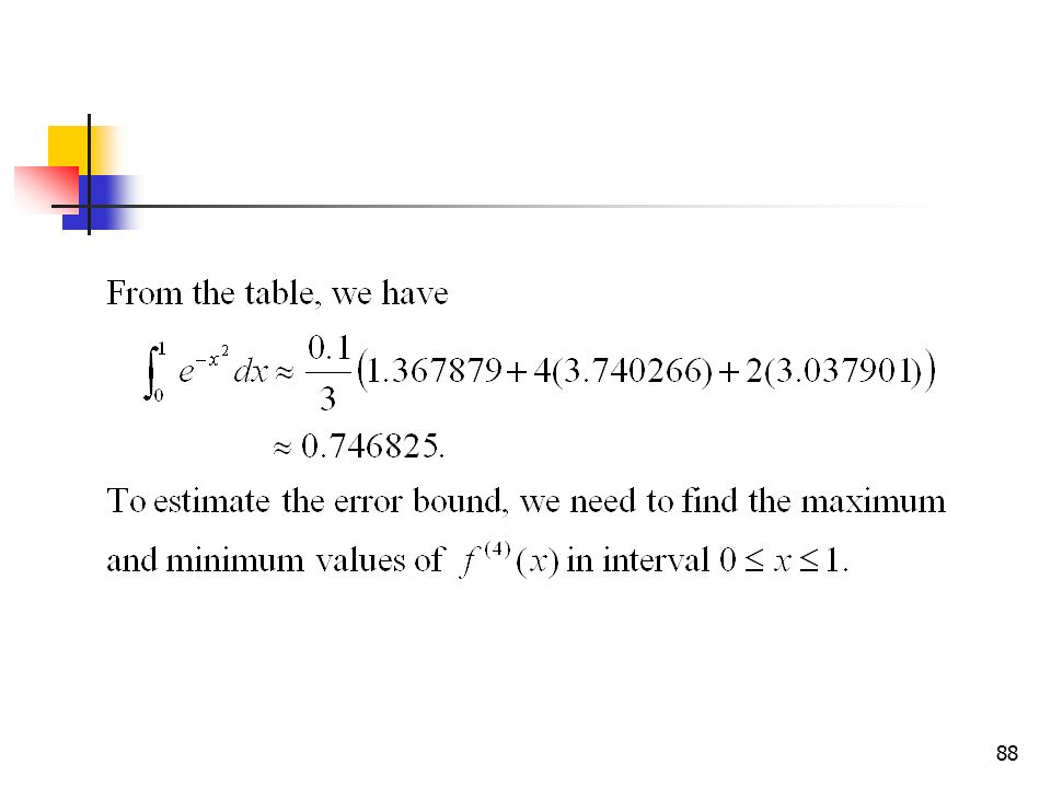
86. Example 3.12
Solution

87. i xi f (a) & f (b) f (xodd) f (xeven) 1 0.1 0.990050 2 0.2 0.960789 31
0.1 2
0.2 3
0.3 4
0.4 5
0.5 6
0.6 7
0.7 8
0.8 9
0.9 10
TOTAL

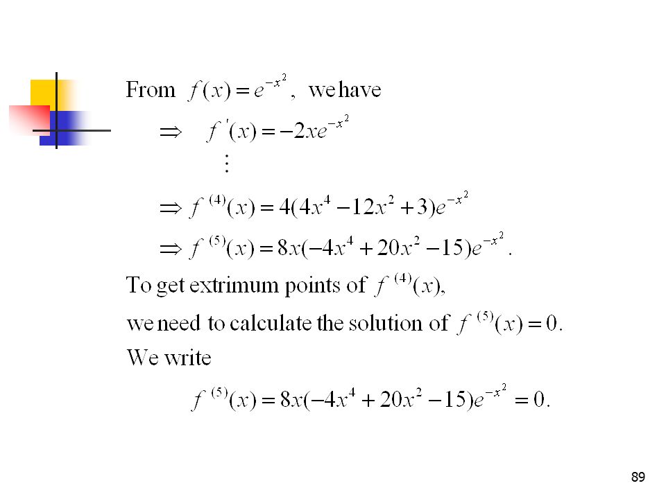
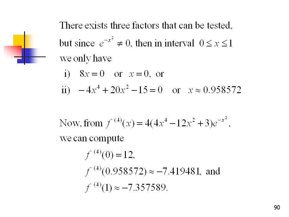
91. O 12  
minimum
maximum
f (4)(x) x 1

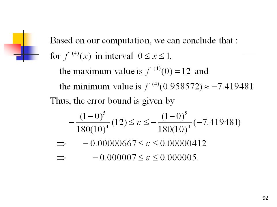
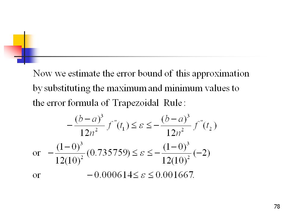
93. error bounds
approximate error bounds

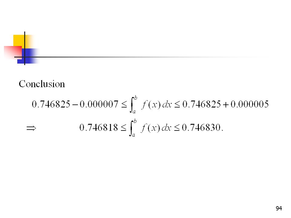
95. 3.4 Numerical Solution of Differential equations
In this part, we discuss two numerical methods to compute approximate solutions of differential equations:
1) One-step Euler method
2) The fourth order Runge-Kutta method

96. NOTATION

97. One-step Euler Method
This method is the most basic numerical method used to solve differential equation.
We shall discuss this Euler Method using the following example:
Example 3.13

98. Solution See the following figure
(x0, y0)
(x1, y1)
4 
1  y x
Figure 3.9 One-step Euler Method with h = 1.

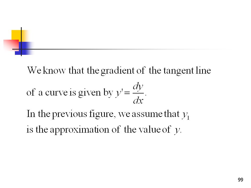
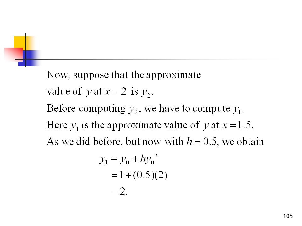
102. Notice that in general, the formula we use to xi yi
yi’ 1 2 3 -
Notice that in general, the formula we use to
estimate y can be written as
The formula of One-step Euler Method

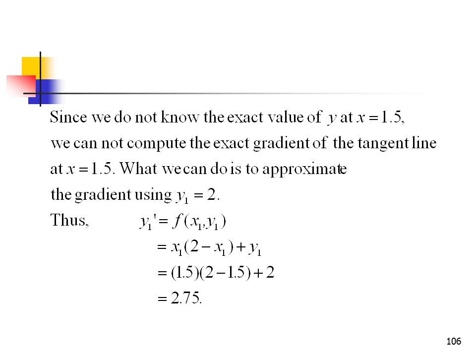
104. See the following figure:
(x0, y0)
(x2, y2)
4 
1  y x
(x1, y1) h
Figure One-step Euler Method with h = 0.5.

107. i xi yi
yi′ 1 2
1.5
2.75
3.375 -

108. NOTATION
Example 3.14

109. Example 3.15
Solution

110. The results of our approximation are listed in the following table:yi
yi’
1.0 1 2
1.2
1.4
2.36
1.872
2.712 3
1.6
2.4144
3.0544 4
1.8 5
2.0 -
Approximation by One-step Euler method with h = 0.2.

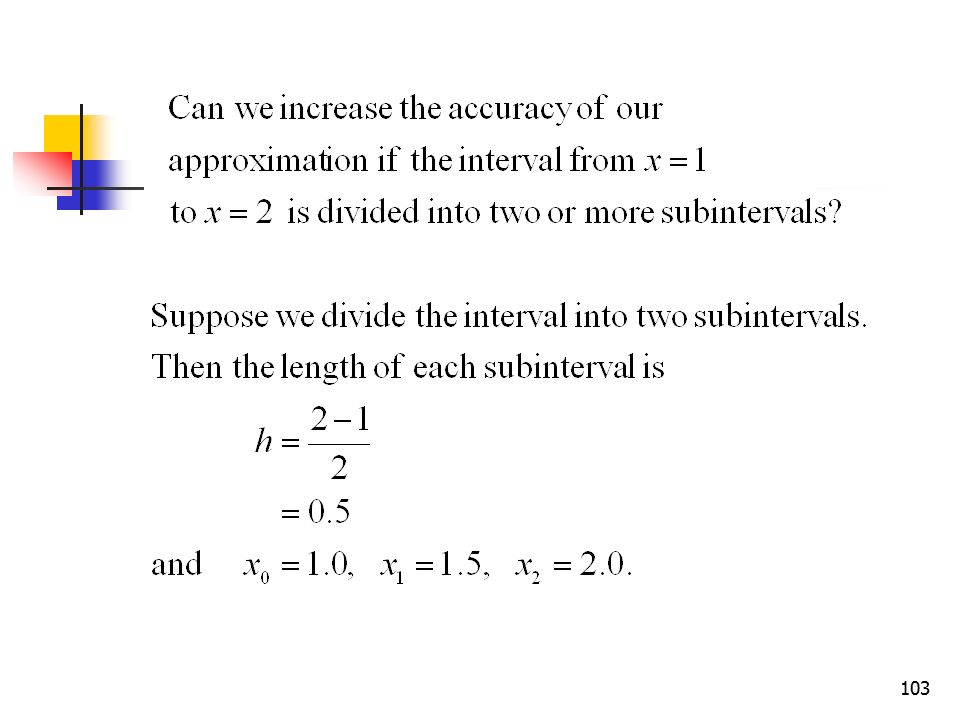
111. If we take ten subintervals, we havexi yi
yi’
1.0 1 2
1.1
1.2
2.19
1.419
2.379 3
1.3
1.6569
2.5669 4
1.4 5
1.5 6
1.6 7
1.7 8
1.8 9
1.9 10
2.0 -
Approximation by One-step Euler method with h = 0.1.

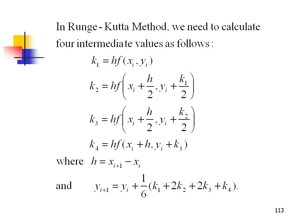
112. 3.4.2 : The fourth order Runge-Kutta Method
Runge-Kutta Method is more accurate compare to Euler Method.
As usual, given y′ = f (x, y) and the initial condition (x0, y0) and we want to find the value of y at other values of x.

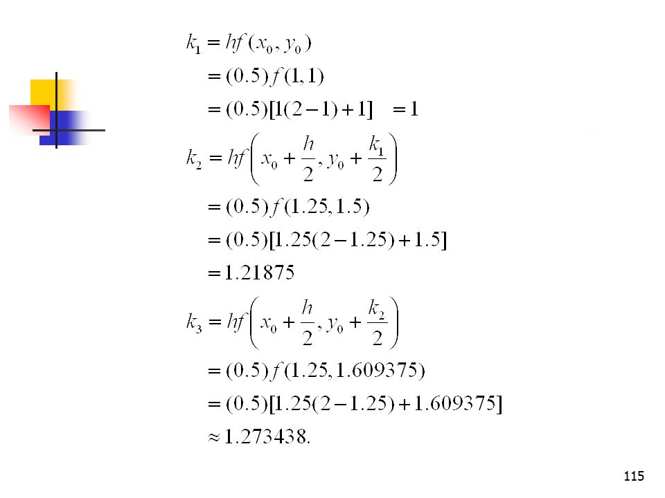
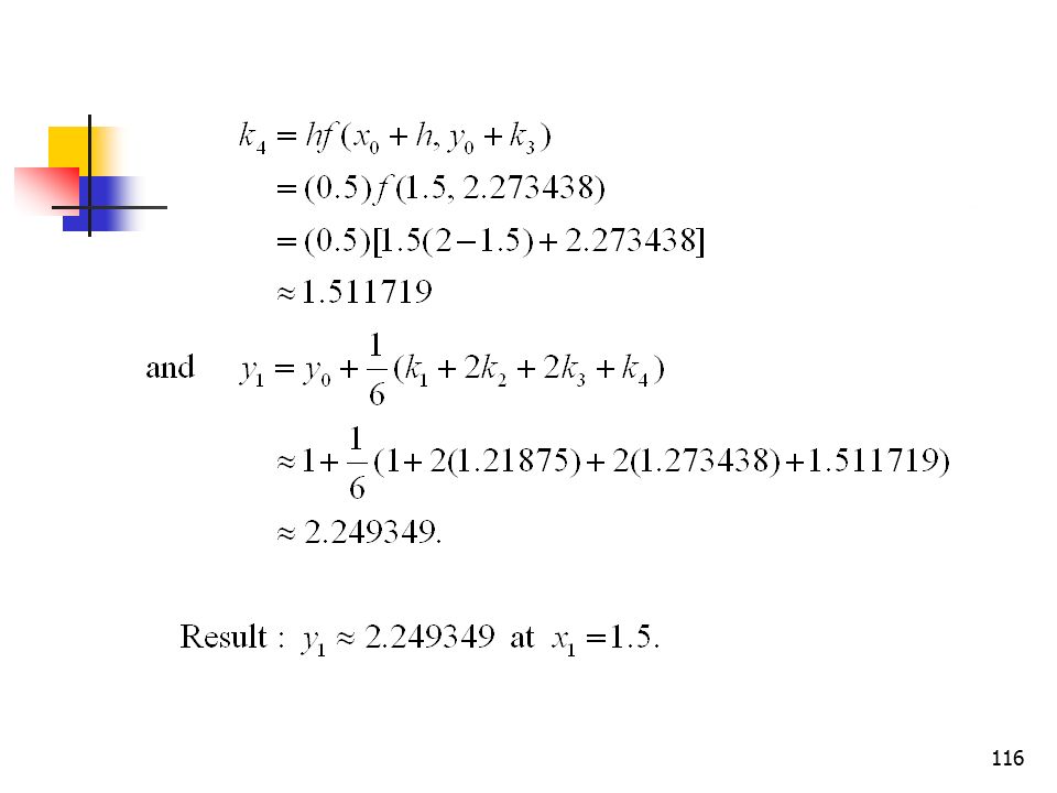
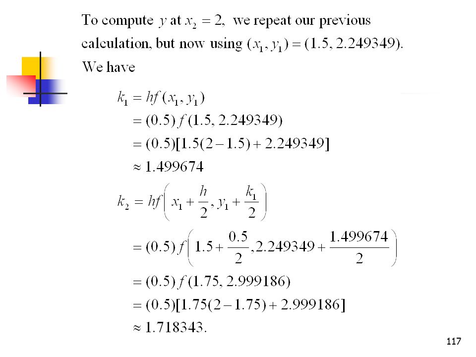
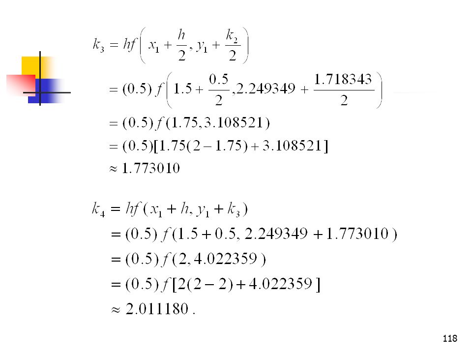
114. Example 3.16
Solution

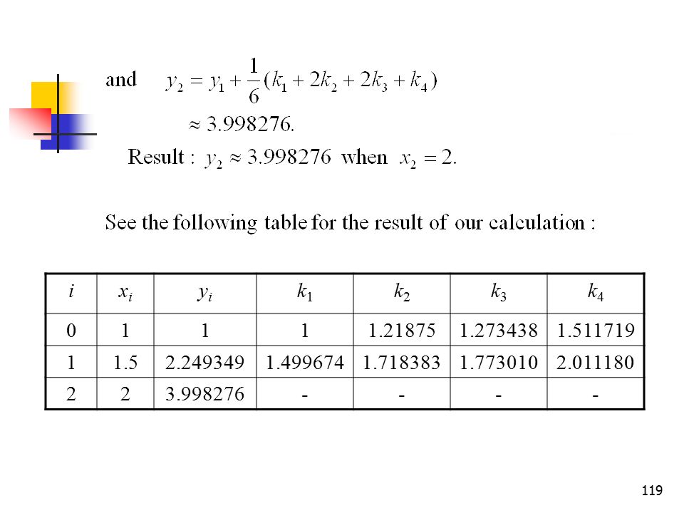
119. i xi yi k1 k2 k3 k4 1
1.5 2 -

120. Conclusion
If we increase the number of subintervals
(i.e. with smaller value of h),
then we obtain a more accurate approximation