1. SIGNALS & SYSTEMS LECTURER: MUZAMIR ISA 049798139muzamir@kukum.edu.myPLV: MUHAMMAD HATTA HUSSEIN 049852853muhdhatta@kukum.edu.my

2. EVALUATION Coursework : 50 % 30 % Practical: 30 % Practical: (i) 70 % from Lab Report (ii) 30% from Lab Test 20 % : 20 % : (i) 15 % from Written Test 1 & Written Test 2 (ii) 5 % from Tutorial Final Exam :50 %

3. REFERENCES Simon Haykin, Barry Van Veen; Signal & System, 2 nd Edition, 2003, Wiley (main textbook) MJ Robert; Signal & System, 2003, McGraw Hill Charles L Philips et.al; Signal, System and Transform, Pearson.

4. Signals and Systems Signals are variable that carry information Signals are variable that carry information Systems process input signals to produce output signals Systems process input signals to produce output signals

5. What Are “Signals”? A function of one or more variable, which conveys information on the nature of a physical phenomenon. A function of time representing a physical or mathematical quantities. e.g. : Velocity, acceleration of a car, voltage/current of a circuit.

6. Even SignalOdd Signal Deterministic Signal Random Signal

7. Classification of Signals Continuous-Time and Discrete-Time Signals Even and Odd Signals Periodic and Nonperiodic Signals Deterministic and Random Signals Energy and Power Signals

8. Continuous Time (CT) and Discrete-Time (DT) Signals

9. Continuous-time signals Continuous-time signals Examples: Signals in cars and circuits Signals described by differential equations, e.g., dy/dt = ay(t) + bf(t) Signal itself could have jumps (discontinuities) in magnitude

10. Discrete-time signals Examples: money in a bank account, daily stock prices No derivative exists Signals described by difference equations, e.g., y(k+1) = ay(k) + bf(k)

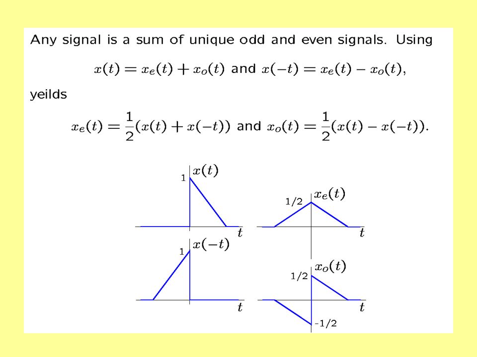
11. Even and Odd Signals

13. Periodic and A-periodic Signals

14. Right and Left-Sided Signals

15. Bounded and Unbounded Signals

16. OPERATION ON SIGNALS Operations performed on the independent variable Time scaling y(t) = x(at) Reflection y(t) = x(-t) Time shifting y(t) = x(t – t 0 ) where t 0 is the time shift.

17. TIME SCALING y(t) = x(at) ; Compress the signal x(t) by a. This is equivalent to plotting the signal x(t) in a new time axis t n at the location given by t = at n or t n = t/a

18. REFLECTION OR FOLDING y(t) = x(- t) Just scaling operation with a = -1. It creates the folded signal x(- t) as a mirror image of x(t) about the vertical axis through the origin t = 0.

19. TIME SHIFTING y(t) = x(t – a) Displaces a signal x(t) in time without changing its shape. Simply shift the signal x(t) to the right by a. This is equivalent to plotting the signal x(t) in a new time axis tn at the location given by t = t n - a or t n = t + a.

20. EXAMPLE A CT signal is shown, sketch and label each of this signal; a) x(t -1) b) x(2t) c) x(-t) 3 2 t x(t)

21. -31 2 t x(-t) 04 t x(t-1) 2 -1/23/2 2 t x(t)

22. A discrete-time signal, x[n-2] A delay by 2 4 2 0 1 2 3 4 5 n x(n-2)

23. A discrete-time signal, x[2n] Down-sampling by a factor of 2. 4 2 0 1 2 3 n x(2n)

24. A discrete-time signal, x[-n+2] Time reversal and shifting 4 2 -1 0 1 2n x(-n+2)

25. A discrete-time signal, x[-n] Time reversal 4 2 -3 -2 -1 0 1 n x(-n)

26. Exercises 1.A continuous-time signal x(t) is shown below, Sketch and label each of the following signal a.x(t – 2)b. x(2t) c.x(t/2)d. x(-t) x(t) t 4 04

27. Continue… 2.A discrete-time signal x[n] is shown below, Sketch and label each of the following signal a. x[n – 2]b. x[2n]c. x[-n+2] d. x[-n] x[n] n 4242 0 1 2 3

28. Basic Operation on Signals Operations performed on dependent variable Amplitude scaling Amplitude scaling Addition Addition Multiplication Multiplication Differentiation Differentiation Integration Integration

29. Exponential Signals x(t) = Be at ; B is the amplitude Decaying Exponential (a < 0) Growing Exponential (a > 0)

30. Sinusoidal Signals x(t) = A cos(  t +  ) where A = amplitude where A = amplitude  = frequency (rad/s)  = frequency (rad/s)  = phase angle (rad)  = phase angle (rad)

31. Unit Impulse Function

32. Narrow Pulse Approximation

33. Intuiting Impulse Definition

34. Uses of the Unit Impulse

35. Unit Step Function

36. Successive Integrations of the Unit Impulse Function