1. Advanced Computer Vision Chapter 3 Image Processing (2) Presented by: 林政安 0932837981 r99944038@ntu.edu.tw 1

2. Image Processing 3.1 Point Operators 3.2 Linear Filtering 3.3 More Neighborhood Operators 3.4 Fourier Transforms 3.5 Pyramids and Wavelets 3.6 Geometric Transformations 3.7 Global Optimization 2

3. 3.5 Pyramids and Wavelets Image pyramids are extremely useful for performing multi-scale editing operations such as blending images while maintaining details. For example, the task of finding a face in an image. Since we do not know the scale at which the face will appear, we need to generate a whole pyramid of differently sized images and scan each one for possible faces. 3

4. 4

5. 3.5.1 Interpolation (Upsampling) Interpolation can be used to increase the resolution of an image. To select some interpolation kernel with which to convolve the image r: upsampling rate. 5

6. 6

7. Bilinear Interpolation 7

8. Bicubic Interpolation Bicubic interpolation – Is an extension of cubic interpolation for interpolating data points on a two dimensional regular grid. – The interpolated surface is smoother than corresponding surfaces obtained by bilinear interpolation. 8

9. 9

10. 3.5.2 Decimation (Downsampling) Decimation is required to reduce the resolution. To perform decimation, we first convolve the image with a low-pass filter (to avoid aliasing) and then keep every rth sample. h(k,l): smoothing kernel 10

11. 11

12. 12

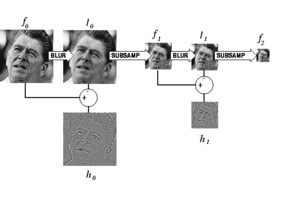
13. 3.5.3 Multi-Resolution Representations Pyramids can be used to accelerate coarse-to- fine search algorithms, to look for objects or patterns at different scales, and to perform multi-resolution blending operations. To construct the pyramid, we first blur and subsample the original image by a factor of two and store this in the next level of the pyramid. 13

14. Gaussian Pyramid (1/2) The technique involves creating a series of images which are weighted down using a Gaussian average and scaled down. Five-tap kernel: 14

15. Gaussian Pyramid (2/2) The reason they call their resulting pyramid a Gaussian pyramid is that repeated convolutions of the binomial kernel converge to a Gaussian 15

16. 16

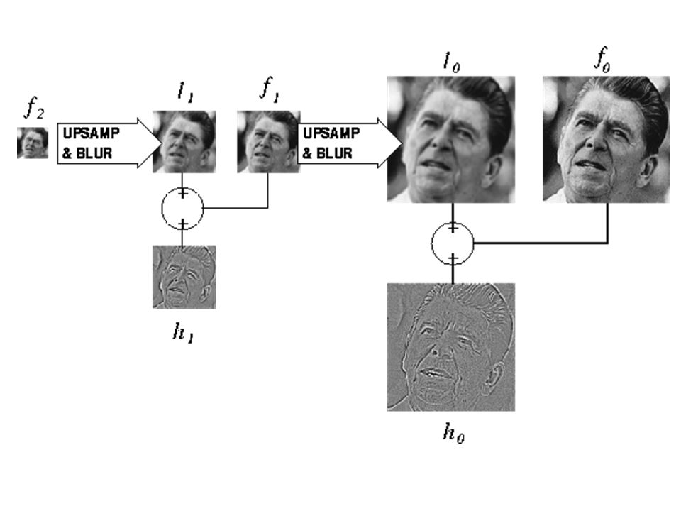
17. Laplacian Pyramid First, interpolate a lower resolution image to obtain a reconstructed low-pass version of the original image. They then subtract this low-pass version from the original to yield the band-pass “Laplacian” image, which can be stored away for further processing. 17

20. Pyramids 20

21. 3.5.4 Wavelets Two-dimensional wavelets The high-pass filter followed by decimation keeps 3/4 of the original pixels, while 1/4 of the low-frequency coefficients are passed on to the next stage for further analysis. The resulting three wavelet images are called the high–high (HH), high–low (HL), and low–high (LH) images. The HL and LH images accentuate the horizontal and vertical edges and gradients, while the HH image contains the less frequently occurring mixed derivatives. 21

22. 22

23. One-Dimensional Wavelets 23

24. Lifted Transform 24

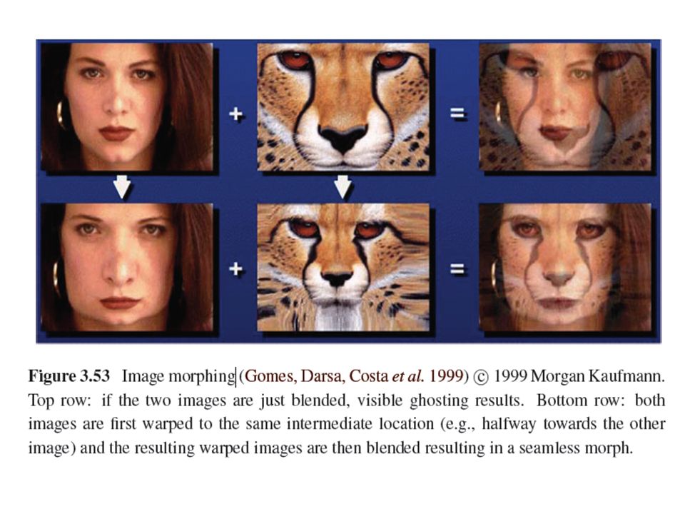
25. Image Blending 25

26. 26

27. 3.6 Geometric Transformations 27

28. 3.6.1 Parametric Transformations Parametric transformations apply a global deformation to an image, where the behavior of the transformation is controlled by a small number of parameters. 28

29. 3.6.1 Parametric Transformations 29

30. Forward Warping The process of copying a pixel f(x) to a location in g is not well defined when has a non-integer value. You can round the value of to the nearest integer coordinate and copy the pixel there, but the resulting image has severe aliasing. The second major problem with forward warping is the appearance of cracks and holes, especially when magnifying an image. 30

31. 31

32. Inverse Warping is (presumably) defined for all pixels in, we no longer have holes. it can simply be computed as the inverse of In fact, all of the parametric transforms listed in Table 3.5 have closed form solutions for the inverse transform: simply take the inverse of the 3 × 3 matrix specifying the transform. 32

33. 33

34. MIP-Mapping (1/3) MIP-mapping was first proposed by Williams (1983) as a means to rapidly pre-filter images being used for texture mapping in computer graphics. A MIP-map is a standard image pyramid, where each level is pre-filtered with a high-quality filter rather than a poorer quality approximation, such as five-tap binomial. 34

35. MIP-Mapping (2/3) To resample an image from a MIP-map, a scalar estimate of the resampling rate r is first computed. Once a resampling rate has been specified, a fractional pyramid level is computed using the base 2 logarithm, 35

36. MIP-Mapping (3/3) One simple solution is to resample the texture from the next higher or lower pyramid level, depending on whether it is preferable to reduce aliasing or blur. Since most MIP-map implementations use bilinear resampling within each level, this approach is usually called trilinear MIP-mapping. 36

37. Anisotropic Filtering An improvement on isotropic MIP mapping Reducing blur and preserving detail at extreme viewing angles 37

38. Multi-Pass Transforms (1/3) The optimal approach to warping images without excessive blurring or aliasing is to adaptively pre-filter the source image at each pixel using an ideal low-pass filter, i.e., an oriented skewed sinc or low-order (e.g., cubic) approximation. 38

39. Multi-Pass Transforms (2/3) 39

40. Multi-Pass Transforms (3/3) For parametric transforms, the oriented two- dimensional filtering and resampling operations can be approximated using a series of one-dimensional resampling and shearing transforms. In order to prevent aliasing, however, it may be necessary to upsample in the opposite direction before applying a shearing transformation. 40

41. 41

42. 3.6.2 Mesh-Based Warping (1/3) While parametric transforms specified by a small number of global parameters have many uses, local deformations with more degrees of freedom are often required. Different amounts of motion are required in different parts of the image. 42

43. 3.6.2 Mesh-Based Warping (2/3) 43

44. 3.6.2 Mesh-Based Warping (3/3) The first approach, is to specify a sparse set of corresponding points. The displacement of these points can then be interpolated to a dense displacement field. A second approach to specifying displacements for local deformations is to use corresponding oriented line segments. 44

46. 3.7 Global Optimization Regularization (variational methods) – Constructs a continuous global energy function that describes the desired characteristics of the solution and then finds a minimum energy solution using sparse linear systems or related iterative techniques. Markov random field – Using Bayesian statistics, modeling both the noisy measurement process that produced the input images as well as prior assumptions about the solution space. 46

47. 3.7.1 Regularization (1/6) 47

48. 3.7.1 Regularization (2/6) Finding a smooth surface that passes through (or near) a set of measured data points. Such a problem is described as because ill- posed many possible surfaces can fit this data. Since small changes in the input can sometimes lead to large changes in the fit, such problems are also often ill-conditioned. 48

49. 3.7.1 Regularization (3/6) Since we are trying to recover the unknown function f(x, y) from which the data point d(x i, y i ) were sampled, such problems are also often called inverse problems. Many computer vision tasks can be viewed as inverse problems, since we are trying to recover a full description of the 3D world from a limited set of images. 49

50. 3.7.1 Regularization (4/6) In order to quantify what it means to find a smooth solution, we can define a norm on the solution space. For one-dimensional functions f(x), we can integrate the squared first derivative of the function, or perhaps integrate the squared second derivative, 50

51. 3.7.1 Regularization (5/6) In two dimensions, the corresponding smoothness functionals are The first derivative norm is often called the membrane, since interpolating a set of data points using this measure results in a tent-like structure. The second-order norm is called the thin-plate spline, since it approximates the behavior of thin plates (e.g., flexible steel) under small deformations. 51

52. 3.7.1 Regularization (6/6) For scattered data interpolation, the data term measures the distance between the function f(x, y) and a set of data points d i =d(x i, y i ) To obtain a global energy that can be minimized, the two energy terms are usually added together, 52

53. 3.7.2 Markov Random Fields (1/3) The posterior distribution for a given set of measurements y, combined with a prior p(x) over the unknowns x, is given by Negative posterior log likelihood. 53

54. 3.7.2 Markov Random Fields (2/3) To find the most likely (maximum a posteriori or MAP) solution x given some measurements y, we simply minimize this negative log likelihood, which can also be thought of as an energy, E d (x, y) is the data energy or data penalty E p (x) is the prior energy

55. 3.7.2 Markov Random Fields (3/3) For image processing applications, the unknowns x are the set of output pixels The data are (in the simplest case) the input pixels

56. 56

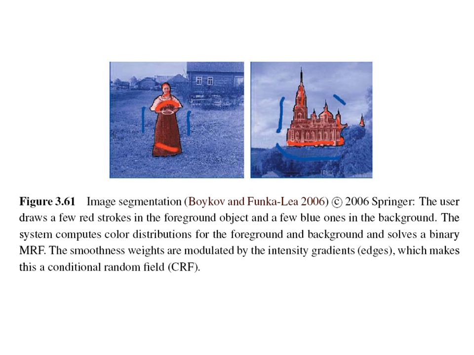
57. Binary MRFs The simplest possible example of a Markov random field is a binary field. Examples of such fields include 1-bit (black and white) scanned document images as well as images segmented into foreground and background regions.

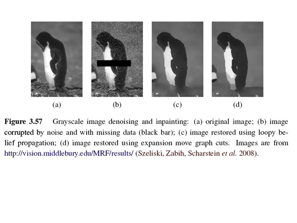
58. Ordinal-Valued MRFs In addition to binary images, Markov random fields can be applied to ordinal-valued labels such as grayscale images or depth maps. The term “ordinal” indicates that the labels have an implied ordering, e.g., that higher values are lighter pixels.

60. Unordered Labels

62. Term Project Tentative term project problems: Exercises in textbook, (30%) total grade: Submit one page in English explaining method, steps, expected results Submit report in a month: April 16 Report progress every other week All right to be the same problem with Master’s thesis

63. Objective: a working prototype with new, original, novel ideas Objective: not just literature survey Objective: not just straightforward implementation of existing algorithms Objective: all right to modify existing algorithms