1. 3D Flow Visualization Xiaohong Ye Email:xhye@soe.ucsc.edu

2.  Flow visualization is useful for several disciplines including: computational fluid dynamics, aerodynamics, turbomachinery design,meteorology and climate modeling. Purposes and Problems of Flow Visualization  Flow visualization in 3D, as opposed to 2D, is more challenging due to perceptual problems such as occlusion,lack of directional cues, lack of depth cues, and visual complexity.

3.  The challenge of 3D visualizations often addressed by selective streamline seeding strategies.  Many of the interesting features of velocity are associated with its critical points. Methods for streamline placement Basic Concepts  Streamline A streamline is an integral curve that is everywhere tangent to a given vector field, such as velocity

4.  Critical points A critical point, also known as a stationary point, is a location in the vector field v where v = 0. Critical points usually are properties investigated in the first place. Examing the neighborhood of the critical points often tells quite important principal characteristics about the entire system behavior. Goal: the visualization does not appear to be cluttered and there are no artifacts introduced in the visualization process 2D Seeding Strategy

5. Image-guided streamline placement Uses a stochastic mechanism to refine the placement of the streamlines. First an initial set of randomly placed streamlines is created. Then this set of streamlines is updated using three valid operations: (1) changing the position and/or length of a streamline, (2) joining streamlines that nearly abut (3) creating a new streamline to fill a gap.

6. An energy function to measure the variation of energy between the current and the updated images Modification is only accepted if the variation of energy is negative. The procedure is iterative the convergence is very slow

7. Procedure: First identify the critical points,locate the position and classify Segment flow field into regions, each contain one critical point each region is seeded with a template Additional seed points are randomly distributed using a Poisson disk Flow-guided streamline placement

8. Different types of critical points in 2D Based on the flow features in the data set Capture flow patterns in the vicinity of critical points non-iterative and view-independent

9. Figure. Seed templates for various critical point. The bold dots represent the seed template and the dashed lines are the streamlines traced using the seed from the template. (a) Center, spiral (b) source, sink (c) saddle

10. Project idea:  Extend the “ flow-guided streamline placement ” on 2D to 3D  Procedure 1. Search the critical points and obtain its position in the object space and classify them. A critical point can be classified according to the eigenvalues of the Jacobi matrix of the vector with respect to position of the critical point.

11. A positive or negative real part of an eigenvalue indicates an attracting or repelling nature. The nonzero imaginary part of eigenvalues create a spiral structure around critical point. We can use Fast to compute the critical points locations and to classify them

12. Three dimensional critical points a)repelling spiral, b) repelling node, c) saddle d) Attracting spiral, repelling in third dimension, e) attracting node, f) center, repelling in the third dimension

13. 2. Streamline seeding We will consider some types of critical points, such as saddle, attracting or repelling spiral In three dimensions, two eigendirections have the same sign and span a plane. The third eigendirection spans a line. Thus, for example v approaches a 3D saddle along a plane and recedes along aline

14. 2. Intergation Equation: S everal integration schemes can be used a. The simplest is the first order Euler technique x(t+Dt) = x(t) + v (x(t)) Dt This approximation is too inaccurate b. I use adaptive fourth-order Runge-Kutta formula

15. Formula: Use of a variable time step, depending on the gradients in the velocity field, is the best solution. This may be done with Dt = a/va, where a is the number of steps per cell, and v a is the average velocity of the eight surrounding grid

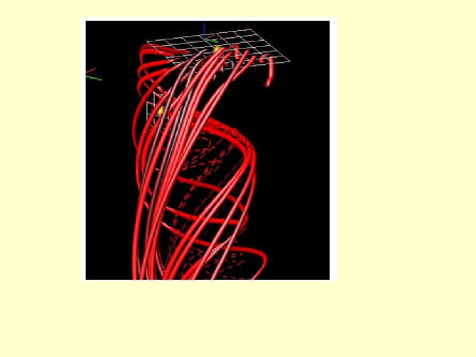
16. 3.Rendering 3D spatial curves are hard to localize without further depth cues. Also, only a small number of curves can be displayed without confusion. Display curves as 3D pipes, allowing occlusion and directional light reflection.

17. References 1.A Flow-guided Streamline Seeding Strategy Vivek Verma, David Kao, Alex Pang IEEE Visualization http://citeseer.nj.nec.com/470972.html 2. Image-Guided Streamline Placement http://www-lil.univ-littoral.fr/~jobard/Research/Publications/EGW- ViSC97/ViSC97.abstract.html 3. A Tool for Visualizing the Topology of Three-Dimensional Vector Fields http://www.nas.nasa.gov/Research/Reports/Techreports/1991/rnr-91-017- abstract.html 4. A Multiresolution Streamlines Seeding Plane http://www.winslam.com/rlaramee/seedingPlane

19. Questions?