1. Summer Inst. Of Epidemiology and Biostatistics, 2008: Gene Expression Data Analysis 8:30am-12:30pm in Room W2017 Carlo Colantuoni – ccolantu@jhsph.edu http://www.biostat.jhsph.edu/GenomeCAFE/GeneExpressionAnalysis/GEA2008.htm

2. Class Outline Basic Biology & Gene Expression Analysis Technology Data Preprocessing, Normalization, & QC Measures of Differential Expression Multiple Comparison Problem Clustering and Classification The R Statistical Language and Bioconductor GRADES – independent project with Affymetrix data. http://www.biostat.jhsph.edu/GenomeCAFE/GeneExpressionAnalysis/GEA2008.htm

3. Class Outline - Detailed Basic Biology & Gene Expression Analysis Technology –The Biology of Our Genome & Transcriptome –Genome and Transcriptome Structure & Databases –Gene Expression & Microarray Technology Data Preprocessing, Normalization, & QC –Intensity Comparison & Ratio vs. Intensity Plots (log transformation) –Background correction (PM-MM, RMA, GCRMA) –Global Mean Normalization –Loess Normalization –Quantile Normalization (RMA & GCRMA) –Quality Control: Batches, plates, pins, hybs, washes, and other artifacts –Quality Control: PCA and MDS for dimension reduction Measures of Differential Expression –Basic Statistical Concepts –T-tests and Associated Problems –Significance analysis in microarrays (SAM) [ & Empirical Bayes] –Complex ANOVA’s (limma package in R) Multiple Comparison Problem –Bonferroni –False Discovery Rate Analysis (FDR) Differential Expression of Functional Gene Groups –Functional Annotation of the Genome –Hypergeometric test?, Χ2, KS, pDens, Wilcoxon Rank Sum –Gene Set Enrichment Analysis (GSEA) –Parametric Analysis of Gene Set Enrichment (PAGE) –geneSetTest –Notes on Experimental Design Clustering and Classification –Hierarchical clustering –K-means –Classification LDA (PAM), kNN, Random Forests Cross-Validation Additional Topics –The R Statistical Language –Bioconductor –Affymetrix data processing example!

4. DAY #2: Intensity Comparison & Ratio vs. Intensity Plots Log transformation Background correction (Affymetrix, 2-color, other) Normalization: global and local mean centering Normalization: quantile normalization Batches, plates, pins, hybs, washes, and other artifacts QC: PCA and MDS for dimension reduction

5. Log Intensity Microarray Data Quantification

6. Log Intensity Log Ratio Microarray Data Quantification

7. Logarithmic Transformation: if : log z (x)=y then : z y =x Logarithm math refresher: log(x) + log(y) = log( x * y ) log(x) - log(y) = log( x / y )

8. Intensity vs. Intensity: LINEAR Intensity Distribution: LINEAR

9. Intensity vs. Intensity: LOG Intensity Distribution: LOG

10. Intensity vs. Intensity: LINEAR

11. Intensity vs. Intensity: LOG

12. Int vs. Int: LINEAR Int vs. Int: LOG Ratio vs. Int: LOG Microarray Data Quantification

13. Background Subtraction

14. Before Hybridization Array 1 Array 2 Sample 1 Sample 2

15. After Hybridization Array 1 Array 2

16. More Realistic - Before Array 1 Array 2 Sample 1 Sample 2

17. Array 1 Array 2 More Realistic - After

18. poly C No label

19. Intensity distributions for the no-label and Yeast DNA

20. The presence of background noise is clear from the fact that the minimum PM intensity is not 0 and that the geometric mean of the probesets with no spike-in is around 200 units. Why Adjust for Background?

21. Local slope decreases as nominal concentration decreases! (E 1 + B) / (E 2 + B) ≈ 1 (E 1 + B) / (E 2 + B) ≈ E 1 / E 2 (E 1 + B) ≈ B or … (E 1 + B) ≈ E 1 or … By using the log-scale transformation before analyzing microarray data, investigators have, implicitly or explicitly, assumed a multiplicative measurement error model (Dudoit et al., 2002; Newton et al., 2001; Kerr et al., 200; Wolfinger et al., 2001). The fact, seen in Figure 2, that observed intensity increase linearly with concentration in the original scale but not in the log-scale suggests that background noise is additive with non-zero mean. Durbin et al. (2002), Huber et al. (2002), Cui, Kerr, and Churchill (2003), and Irizarry et al. (2003a) have proposed additive-background-multiplicative-measurement-error models for intensities read from microarray scanners.

22. Affymetrix GeneChip Design 5’ 3’ Reference sequence …TGTGATGGTGCATGATGGGTCAGAAGGCCTCCGATGCGCCGATTGAGAAT… GTACTACCCAGTCTTCCGGAGGCTA GTACTACCCAGTGTTCCGGAGGCTA Perfectmatch (PM) Mismatch (MM) NSB & SB NSB

23. Why not subtract MM?

26. Background: Solutions

27. Affymetrix GeneChip Design 5’ 3’ Reference sequence …TGTGATGGTGCATGATGGGTCAGAAGGCCTCCGATGCGCCGATTGAGAAT… GTACTACCCAGTCTTCCGGAGGCTA GTACTACCCAGTGTTCCGGAGGCTA Perfectmatch (PM) Mismatch (MM) NSB & SB NSB

28. Motivation: PM - MM PM = B + S MM = B PM – MM = S The hope is that: But this is not correct!

29. Simulation We create some feature level data for two replicate arrays Then compute Y=log(PM-kMM) for each array We make an MA using the Ys for each array We make a observed concentration versus known concentration plot We do this for various values of k. The following “movie” shows k moving from 0 to 1.

30. k=0 Known level (log2) Observed level (log2) Log2(Intensity) Log2(Ratio)

31. k=1/4 Known level (log2) Observed level (log2) Log2(Intensity) Log2(Ratio)

32. k=1/2 Known level (log2) Observed level (log2) Log2(Intensity) Log2(Ratio)

33. k=3/4 Known level (log2) Observed level (log2) Log2(Intensity) Log2(Ratio)

34. k=1 Known level (log2) Observed level (log2) Log2(Intensity) Log2(Ratio)

35. Real Data MAS 5.0RMA

36. RMA: The Basic Idea PM=B+S Observed: PM Of interest: S Pose a statistical model and use it to predict S from the observed PM

37. The Basic Idea PM=B+S A mathematically convenient, useful model –B ~ Normal ( ,  ) S ~ Exponential ( ) –No MM –Borrowing strength across probes

39. MAS 5.0

40. RMA Notice improved precision but worse accuracy

41. Problem Global background correction ignores probe-specific NSB MM have problems Another possibility: Use probe sequence

42. Probe-specific Background

43. G-C content effect in PM’s Boxplots of log intensities from the array hybridized to Yeast DNA for strata of probes defined by their G-C content. Probes with 6 or less G-C are grouped together. Probes with 20 or more are grouped together as well. Smooth density plots are shown for the strata with G-C contents of 6,10,14, and 18. Any given probe will have some propensity to non-specific binding. As described in Section 2.3 and demonstrated in Figure 3, this tends to be directly related to its G-C content. We propose a statistical model that describes the relationship between the PM, MM, and probes of the same G-C content.

44. General Model (GCRMA) NSBSB We can calculate: Due to the associated variance with the measured MM intensities we argue that one data point is not enough to obtain a useful adjustment. In this paper we propose using probe sequence information to select other probes that can serve the same purpose as the MM pair. We do this by defining subsets of the existing MM probes with similar hybridization properties.

45. The MA plot shows log fold change as a function of mean log expression level. A set of 14 arrays representing a single experiment from the Affymetrix spike-in data are used for this plot. A total of 13 sets of fold changes are generated by comparing the first array in the set to each of the others. Genes are symbolized by numbers representing the nominal log2 fold change for the gene. Non-differentially expressed genes with observed fold changes larger than 2 are plotted in red. All other probesets are represented with black dots. The smooth lines are 3SDs away with SD depending on log expression.

47. Naef & Magnasco (2003), PHYSICAL REVIEW E 68, 011906, 2003 Another sequence effect in PM’s and MM’s

48. We show in Fig. 2 joint probability distributions of PMs and MMs, obtained from all probe pairs in a large set of experiments. Actually, two separate probability distributions are superimposed: in red, the distribution for all probe pairs whose 13th letter is a purine, and in cyan those whose 13 th letter is a pyrimidine. The plot clearly shows two distinct branches in two colors, corresponding to the basic distinction between the shapes of the bases: purines are large, double ringed nucleotides while pyrimidines have smaller single rings. This underscores that by replacing the middle letter of the PM with its complementary base, the situation on the MM probe is that the middle letter always faces itself, leading to two quite distinct outcomes according to the size of the nucleotide. If the letter is a purine, there is no room within an undistorted backbone for two large bases, so this mismatch distorts the geometry of the double helix, incurring a large steric and stacking cost. But if the letter is a pyrimidine, there is room to spare, and the bases just dangle. The only energy lost is that of the hydrogen bonds. Naef & Magnasco (2003), PHYSICAL REVIEW E 68, 011906, 2003

49. C and T are pyrimidines (and small), A and G are purines (and large).

50. Why not subtract MM?

51. Another sequence effect in PM’s Naef & Magnasco (2003), PHYSICAL REVIEW E 68, 011906, 2003 The asymmetry of (A,T) and (G,C) affinities in Fig. 3 can be explained because only A-U and G-C bonds carry labels ~purines U and C on the mRNA are labeled. Notice the nearly equal magnitudes of the reduction in both type of bonds. (Remember also that G-C pairs have 3 and A-T pairs have 2 hydrogen bonds!).

52. Two color platforms (Agilent, cDNA) Common to have just one feature per gene 60 vs. 25 NT? Optical noise still a concern After spots are identified, a measure of local background is obtained from area around spot (this is also applicable to some spotted one-channel data)

53. Local background ---- GenePix ---- QuantArray ---- ScanAnalyze

54. Two color feature level data Red and Green foreground and background obtained from each feature We have Rf gij, Gf gij, Rb gij, Gb gij (g is gene, i is array and j is replicate) A default summary statistic is the log-ratio: log 2 [(Rf-Rb) / (Gf - Gb)]

55. Background subtraction No background subtraction

56. Diagnostics: images of Rb, Gb, scatterplot of log2 (Rf/Gf) vs. log2(Rb/Gb)

57. Correlation may be spatially dependent

58. Two color platforms Again, we can assess the tradeoff of accuracy and precision via simulation Simulation uses a self versus self (SVS) hybridization experiment -- no differential expression should occur. Mean squared error (MSE) = bias^2 + variance.

59. Lower MSE with NBS if correlation < 0.2

60. A procedure that subtracts local background as a function of the correlation of fg and bg ratios may be a nice compromise between background subtraction and no background subtraction. For references, see background subtraction paper by C. Kooperberg J Computational Biol 2002. Limma package in R has many useful functions for background subtraction. Following the decision to background subtract, we need to consider a normalization algorithm. Background Subtraction: Conclusions

61. Normalization

62. Normalization is needed to ensure that differences in intensities are indeed due to differential expression, and not some printing, hybridization, or scanning artifact. Normalization is necessary before any analysis which involves within or between slides comparisons of intensities, e.g., clustering, testing. Somewhat different approaches are used in two-color and one-color technologies

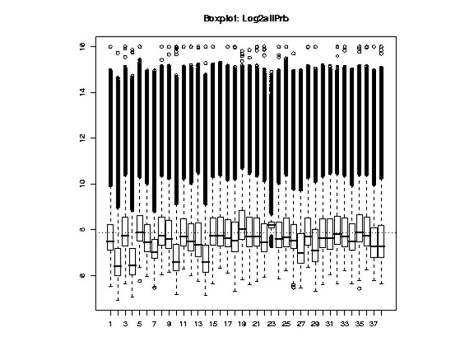
63. Varying distributions of intensities from each microarray.

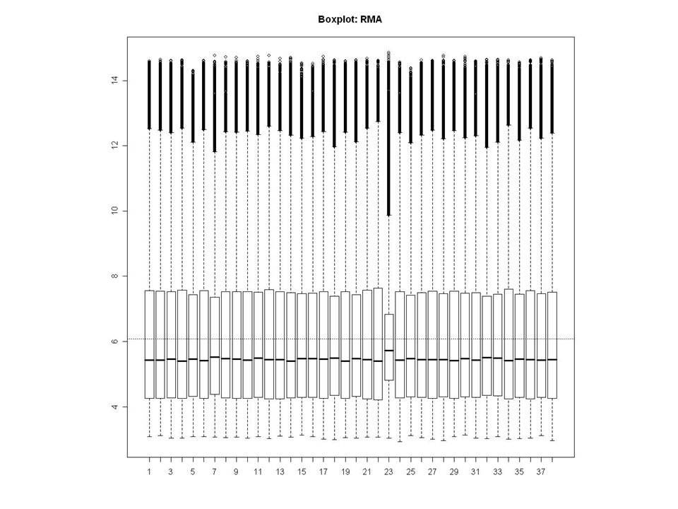
64. Distributions of intensities after global mean normalization.

65. What does this normalization mean in Int vs. Int, or Ratio vs. Int space?

66. Distributions of intensities after global mean normalization – global mean normalization is not enough … Possible solutions: Local Mean Normalization Quantile Normalization

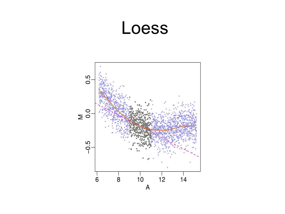
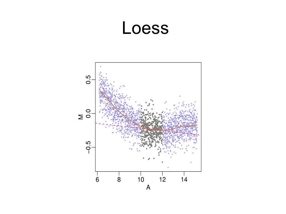
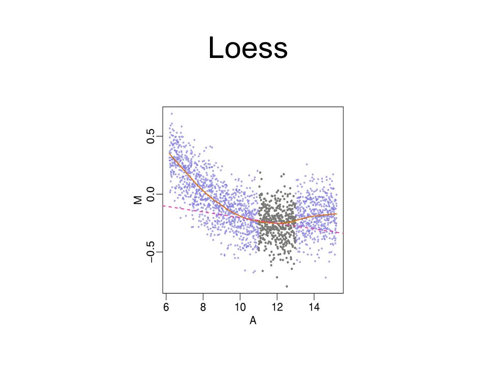
67. Local Mean Normalization (loess): Adjusts for intensity- dependent bias in ratios. Requires Comparison!

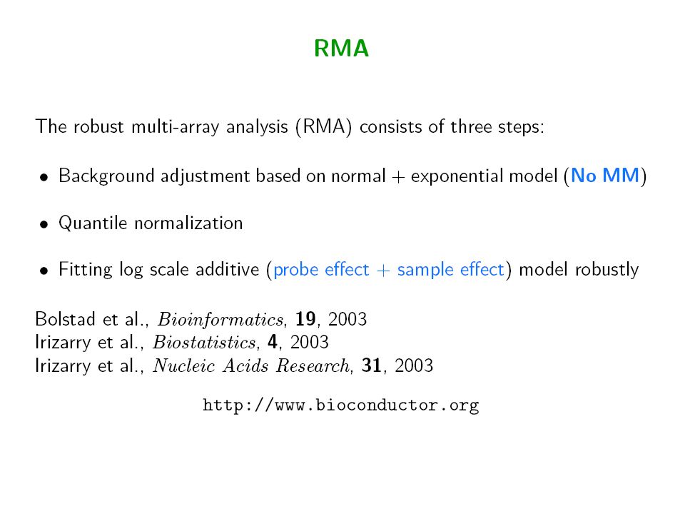
70. Loess

76. Quantile Normalization

77. Quantile normalization All these non-linear methods perform similarly Quantiles is commonly used because its fast and conceptually simple Basic idea: –order value in each array –take average across probes –Substitute probe intensity with average –Put in original order

78. Example of quantile normalization 244 5414 468 358 339 234 348 348 459 56 333 555 555 666 888 353 858 685 565 536 OriginalOrderedAveragedRe-ordered

79. Before Quantile Normalization

80. After Quantile Normalization A worry is that it over corrects

81. QC

86. Print-tip Effect

87. Print-tip Loess

88. Plate effect

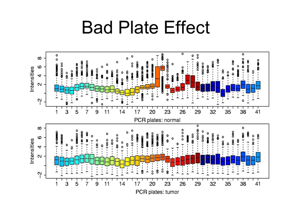
89. Bad Plate Effect

91. Print Order Effect

92. Microarray Pseudo Images: Intensity

93. Microarray Pseudo Images: Ratios

94. Images of probe level data This is the raw data

95. Images of probe level data Residuals (or weights) from probe level model fits show problem clearly

96. Hybridization Artifacts

99. PCA, MDS, and Clustering: Dimension Reduction to Detect Experimental Artifacts and Biological Effects

100. Principle Components Analysis (PCA) and Multi-Dimensional Scaling (MDS)

101. PCA

102. MDS

107. Uncorrected Intensities: MDS Colored by Batch

108. Removing The Batch Effect Much Like Red:Green Analysis

109. Uncorrected Intensities: MDS Colored by Batch

110. Batch Subtracted Measures: MDS Colored by Batch

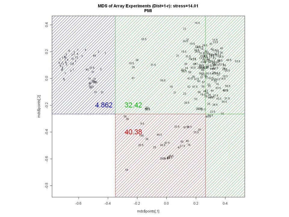
111. MDS of All Array Experiments: Subject Replicates

113. AGE ?

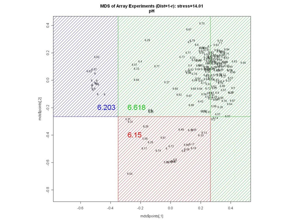
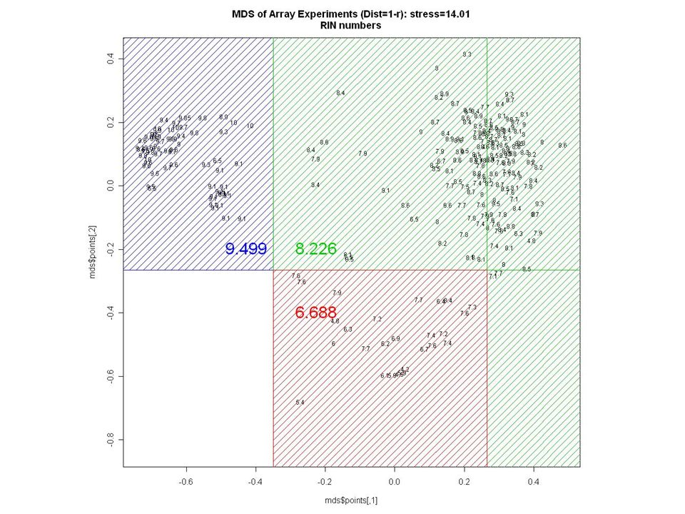
121. RNA Quality

122. AGE Batch

124. Biological Effects: Tissue Types and Growth Factor Treatments

125. Illumina 24K