Download presentation
Presentation is loading. Please wait.

1
Seismic measurements of stellar rotation with Corot: theoretical expectations and HH results Goupil, Samadi, Barban, Dupret, (Obs. Paris) Appourchaux (IAS) and Corot sismo HH3 group 1. What can we expect upon detection, precision of splitting measurements ? 2. Illustration : results from one HH exercise: HD 49933 3. What amount of information upon rotation can we expect?
 Appourchaux (IAS) and Corot sismo HH3 group 1. What can we expect upon detection, precision of splitting measurements . 2. Illustration : results from one HH exercise: HD What amount of information upon rotation can we expect .")
2
An oscillating star: time variability L(t) --> power spectrum nlm = frequency for a given oscillation mode: n, l, m (l,m from a description with spherical harmonics Y lm ) No rotation : nl a 2l+1 degenerate mode (m=-l, l) Rotation ( ) breaks the azimuthal symetry, lifts the degeneracy: 2l+1 modes (given n,l): Rotational splitting: nlm nlm - nl to be measured -m m
 --> power spectrum nlm = frequency for a given oscillation mode: n, l, m (l,m from a description with spherical harmonics Y lm ) No rotation : nl a 2l+1 degenerate mode (m=-l, l) Rotation ( ) breaks the azimuthal symetry, lifts the degeneracy: 2l+1 modes (given n,l): Rotational splitting: nlm nlm - nl to be measured -m m ")
3
splitting rotation rate nlm = m r K nl (r, ) d dr (K nl rotational kernel ) = m s C nl if uniform rotation measured deduced
 d dr (K nl rotational kernel ) = m s C nl if uniform rotation measured deduced")
4
Two cases: Opacity driven oscillations: Scuti, Cep, Dor.., masses > ~ 1.5 Msol Large amplitudes, fast rotators, infinite lifetime: 'zero' width Detection, precision : easy but who is who ? Mode identification pb Stochastically excited, damped oscillations: solar like : Sun, a Cen, Procyon, n Boo, HD49933 Small amplitude, 'slow' rotators, finite lifetime: width Detection? precision ? A damped triplet l=1 modes: Resolved tripletNon resolved triplet

5
Signal to noise ratio SNR Splitting : width T :observing time interval How many splittings, what precision for what star? Detection criterion: SNR > 9 and > 1 + 0 /2 ~ 0 Precision : ( T/ ) f(SNR) (Libbrecht 92)
 f(SNR) (Libbrecht 92).")
6
SNR = funct(A 1, noise level (app. mag(distance)) ) (SNR = SNR 0 10 ( m-5.7 ) ; SNR 0 = funct(A 1, ) (Corot specification) ) A 1 /A 0 = funct(visibility (inclination angle)) A 0, 0 = funct(mass, age) T = 150 days or 20 days observing time interval = funct( ) Input: mass(luminosity), age (T eff ), distance, ,i, T Output: splitting detected, precision of measurement How many splittings, what precision for what star? Detection criterion: SNR > 9 and > 1 + 0 /2 ~ 0 Precision: ( T/ ) f(SNR) (Libbrecht 92)
) ) (SNR = SNR 0 10 ( m-5.7 ) ; SNR 0 = funct(A 1, ) (Corot specification) ) A 1 /A 0 = funct(visibility (inclination angle)) A 0, 0 = funct(mass, age) T = 150 days or 20 days observing time interval = funct( ) Input: mass(luminosity), age (T eff ), distance, ,i, T Output: splitting detected, precision of measurement How many splittings, what precision for what star. Detection criterion: SNR > 9 and > 1 + 0 /2 ~ 0 Precision: ( T/ ) f(SNR) (Libbrecht 92).")
7
Selected models in HR diagram: 4 TAMS models and one ZAMS model, p3Ori 1.2 Mo 1.3Mo 1.4 Mo Signal to Noise Ratio Number of detected splittings increases with mass and age

8
LRa1 sismo B2III Be F0V solar-like G0 solar-like B0.5V F1V B9V B9ApV G5II F2V B8IV 5.5<mv<9.5

9
width Hz (for v=10,20,30 km/s) 3 Ori v=10 km/s v=20km/s v=30 km/s Uncertainty of splitting measurement ( Hz) Colours correspond to detected splittings for different inclination angle Number of detected splittings increase with i
 3 Ori v=10 km/s v=20km/s v=30 km/s Uncertainty of splitting measurement ( Hz) Colours correspond to detected splittings for different inclination angle Number of detected splittings increase with i ")
10
Illustrative case: HH3 HD49933 (1.4 M sol, 6700 K) Target for Corot --> HH exercise --> Observed from ground with Harps(Mosser et al 2005): detection of solar like oscillation Many splittings detected. Only a few correct within 0.5 Hz and with error bars < 0.5 Hz Differences between input splitting values from simulation (Roxburgh, Barban) and output splitting values from blind analysis (Appourchaux)
 and output splitting values from blind analysis (Appourchaux).")
12
3 levels: level 1: Only a few modes P rot as an average: P rot -1 = (1/N) j=1,N ( j + j ) level 2: Enough splittings with enough precision for a forward indication of r-variation rotation profile (r) level 3: Enough accurate splittings with appropriate nature for successful inversion process 3. What amount of information upon rotation ?

13
V rot =13 km/s V rot = 30 km/s Level 2: ( Hz) Uncertainty for detected splittings Hz Splitting with uniform rotation with r c s Colors = different inclination angle i
 Uncertainty for detected splittings Hz Splitting with uniform rotation with r c s Colors = different inclination angle i")
14
Blue: 1.5 M sol TAMS model i > 60° v =30 km/s Red: 1.3 M sol TAMS model level 1 level 2 level 3 P rot,split - P rotsurfture ~ a few hours For nonuniform rotation P rotsurfture ~ days core / surf ~ 2 uncertainties P rot/ P rot ~10 -4

15
Summary Pessimist view : Testing rotation analogous to the solar case is going to be difficult Instrumental noise, stellar activity 'noise' not included Optimist view: Assumed core / surf ~ 2 seems to be conservative, underestimation Most favorable cases: relatively massive (1.4-1.6 Msol), cool, brightest, relatively high v sin i (high v and/or high i) ~ 5 Corot stars for inversion ( (r) ) (Lochard, 2005) ~ perhaps a few 10 for forward technique (hint for (r) ) ~ a few more for Prot (but independent of activity, spots)
, cool, brightest, relatively high v sin i (high v and/or high i) ~ 5 Corot stars for inversion ( (r) ) (Lochard, 2005) ~ perhaps a few 10 for forward technique (hint for (r) ) ~ a few more for Prot (but independent of activity, spots)")
21
Summary

24
How seismology can help infer information on rotation (and related processes) Ultimate goal: determine (r, ,t) from PMS to compact object for small to large mass star s COROT: significant advances in the field expected Goupil, MJ, Observatoire de Paris Lochard J., Samadi R., Moya A., Baudin F., Barban C., Baglin A. French-spanish connection: Suarez JC., Dupret M., Garrido R.

25
One info ( P rot surf ) -- many stars Statistical studies: relations rotation - others quantities 1. Rotation- light elements abundance- convection ---------->> José Dias do Nascimento 2. Age - rotation (v sin i) in young clusters 3. Rotation (Rossby number) – activity relation (periodic variability)
 in young clusters 3. Rotation (Rossby number) – activity relation (periodic variability).")
26
to day COROT Activity level photometric variability 10 -2 -3 10 -4 -5 versus Stellar parameters convection, rotation, Ro P rot Extension of the knowledge of magentic activity to stars earlier than G8 Sun Ground observations Precision 10 -2 From A. Baglin 3. Rotation (Rossby number) – activity relation (periodic variability)
 – activity relation (periodic variability).")
27
1. Measurements of v sin i ( Royer et al 2002; Custiposto et al 2002 ) A, B stars v sin i (km/s) 100 F G K 30 10 v sin i (km/s) Histograms:
 A, B stars v sin i (km/s) 100 F G K v sin i (km/s) Histograms:.")
28
2. Determination of surface rotation period: P rot Detection of spots, activity level Latitude differential rotation ( Petit et al 2004, Donati et al 2003, Reiners et al 2003, Strassmeier 2004) MS massive stars (9 -20 M sol ): Meynet, Maeder (04) evolution of surface rotation affected by mass loss and internal transport mechanisms v/v crit ~ 0.9 ( Townsend et al. 04 ) --> v esc ~c s nonradial puls. driven wind ( Owocki 04 ) --> AM Hubert Mass loss or transport mechanism is dominant in influencing Prot depending on the mass of the star (M >12 <12Msol) Determination of P rot versus distance from the ZAMS
 MS massive stars (9 -20 M sol ): Meynet, Maeder (04) evolution of surface rotation affected by mass loss and internal transport mechanisms v/v crit ~ 0.9 ( Townsend et al. 04 ) --> v esc ~c s nonradial puls. driven wind ( Owocki 04 ) --> AM Hubert Mass loss or transport mechanism is dominant in influencing Prot depending on the mass of the star (M >12 <12Msol) Determination of P rot versus distance from the ZAMS.")
29
One star -- many periods Seismology : rotation Depth dependence (r) : 2 extreme cases: * uniform rotation * conservation of local angular momentum Reality is somewhere in-between depending on the mass and age of the star Diagnostic of transport processes inside stars
 : 2 extreme cases: * uniform rotation * conservation of local angular momentum Reality is somewhere in-between depending on the mass and age of the star Diagnostic of transport processes inside stars")
30
(t) = J(t) / I(t) Rotation profile inside a star is representative of redistribution of angular momentum J from one stellar region to another : caused by evolution: contractions and dilatations of stellar regions: I(t) caused by dynamical and thermal instabilities: meridional circulation, differential rotation and turbulence: J(t) caused by surface losses by stellar winds (B, thermal) or surface gain by interaction with surrounding : J(t) These processes cause chemical transport which in turn affects the structure and evolution of the star
 = J(t) / I(t) Rotation profile inside a star is representative of redistribution of angular momentum J from one stellar region to another : caused by evolution: contractions and dilatations of stellar regions: I(t) caused by dynamical and thermal instabilities: meridional circulation, differential rotation and turbulence: J(t) caused by surface losses by stellar winds (B, thermal) or surface gain by interaction with surrounding : J(t) These processes cause chemical transport which in turn affects the structure and evolution of the star")
31
We want to identify region of uniform rotation and region of differential rotation (depth, latitude dependence) inside the star ( core/ surf) This depends on the type of star
 inside the star ( core/ surf) This depends on the type of star")
32
Small and intermediate mass main sequence stars Intermediate and large mass (OBA) stars: no or thin external convective zone --> no loss of angular momentum --> intermediate and fast rotators Schematically : PMS stars: I varies a lot Small mass (FGK) stars – : external convective zone --> stellar wind - magnetic breaking --> loss of angular momentum --> slow rotators COROT will tell: a bit too simplified view !!!
 stars: no or thin external convective zone --> no loss of angular momentum --> intermediate and fast rotators Schematically : PMS stars: I varies a lot Small mass (FGK) stars – : external convective zone --> stellar wind - magnetic breaking --> loss of angular momentum --> slow rotators COROT will tell: a bit too simplified view !!!")
33
Determination of rotation profile: seismic diagnostics with forward and inversion techniques Forward: compute from a model, given and compare with obs Inversion: compute < r from appropriate combinations of { obs }

34
Solar Case Latitudinal in convective region: B, tachocline Uniform in radiative region: transport of J : meridional circulation + turbulent shear : not sufficient add B ? (Zahn and Co) Result from inversion Tachocline: new abundances sound speed inversion : needs rotational mixing ? Give hints what to search for other stars
 Result from inversion Tachocline: new abundances sound speed inversion : needs rotational mixing . Give hints what to search for other stars.")
35
Solar-like Oscillations (F-G-K ) A ~ cm/s to ~ m/s P ~ min-h from C. Barban & MA Dupret Cephei Scuti Doradus WD OTHER STARS

36
Other stars other problems ! Unknown : mass, age, X, Z,, i physics, (n,l,m) new philosophy Efforts developed from ground: we must use multisite observations, multitechniques, i.e. use seismic and non seismic information To built a seismic model (non unique solution) ( determine all unknown quasi at the same time ) serves at improving -determination of stellar parameters ie ages -test different physical prescriptions gives a model closer to reality for iteration and inversion techniques
 new philosophy Efforts developed from ground: we must use multisite observations, multitechniques, i.e. use seismic and non seismic information To built a seismic model (non unique solution) ( determine all unknown quasi at the same time ) serves at improving -determination of stellar parameters ie ages -test different physical prescriptions gives a model closer to reality for iteration and inversion techniques.")
37
Axisymetric --> (r, ) --> (r) = horiz We must distinguish fast, moderate and slow rotators : = G R 3 ) centrifugal over gravitational = / coriolis / oscillation period - Slow ( <<1 ) : first order perturbation is enough - Intermediate ( ~ < 0.5) : higher order contributions necessary - Fast ( > 0.5) : 2D eq. models + nonperturbative osc. app.

38
- diagram Rapid rotation: structure: oblatness, meridional circulation, chemical mixing : large Slow rotation but / large moderate small fast

39
Then the linear splitting is: Frequency of the component m of a multiplet of modes (n,l) no rot Coriolis 1st order contr. Surface rotation rate If uniform, then m /C = is constant, V m Generalized splitting: m m = m - (-m) m m = 0 + m surf C
 m m = 0 + m surf C.")
40
Variable white dwarfs PG1159-035 oscillate with asymptotic g modes Mode identification rather easily Many l=1 triplets and l=2 multiplets Weakly sensitive to depth variation of DBV GD358: Non uniform (depth) rotation: Winget et al 1991 Winget et al 1994 --> Kepler
 rotation: Winget et al 1991 Winget et al > Kepler")
41
A, B type stars Extension of mixed inner region for rotating convective core ? overshoot + rotation will depend on the type of stars, on each star ? a slow rotator Cepheid a Dor star : small but also ! Rapid rotators : Scuti type (PMS, MS, post MS) v sin i= 70-250 km/s =up to 0.3 Not discussed here : Ro Ap stars slow rotators but indirect effect of rotation Rapid rotators B, Be ---> A.M. Hubert
 v sin i= km/s =up to 0.3 Not discussed here : Ro Ap stars slow rotators but indirect effect of rotation Rapid rotators B, Be ---> A.M. Hubert.")
42
Rotating convective core is prolate Rotating convective core of A stars 3 D simulations (Browning et al 2004) 2 M sol ; rotation 1/10 to 4 times sol Differential rotation ( )for convective core Heat (enthalpy) flux increases --> larger mixed region r c = 0.1 R* r 0 = 0.15 R*
 2 M sol ; rotation 1/10 to 4 times sol Differential rotation ( )for convective core Heat (enthalpy) flux increases --> larger mixed region r c = 0.1 R* r 0 = 0.15 R*")
43
* a Cepheid HD 129929 : (Dupret et al 04; Aerts et al 04) Lot of effort ! : multisite observations + multitechniques then frequencies + location in HR diagram + mode identification (l degree) + nonadiabatic (n order) then Seismic models can be built A triplet l=1 and some l=2 components yield : d ov = 0.1 +_ 0.05 core / surf = 3.6 --> Core rotates faster than envelope (Ps = 140 d; surface 2 km/s) 4 frequencies : no standard model fits, asymetric multiplets core = 3 surf (Pamyatnykh et al 2004) but 2 different studies: different conclusions ---->> Nonstandard physics in stellar models: diffusion, rotational distorsion Eri (Ausseloos et al 2004)
 + nonadiabatic (n order) then Seismic models can be built A triplet l=1 and some l=2 components yield : d ov = 0.1 +_ 0.05 core / surf = > Core rotates faster than envelope (Ps = 140 d; surface 2 km/s) 4 frequencies : no standard model fits, asymetric multiplets core = 3 surf (Pamyatnykh et al 2004) but 2 different studies: different conclusions ---->> Nonstandard physics in stellar models: diffusion, rotational distorsion Eri (Ausseloos et al 2004).")
44
Long oscillation periods: g modes: asymptotics yields radial order Seismic models can be built (non unique) (v sin i 53-66 km/s; Prot =1,15 d) use mode excitation (nonadiabatic) information but must take into account effects of large ( Dintrans, Rieutord,2000) P < 3 days second order pert. tech no longer valid D a Dor (Moya et al. 2004)
.")
45
spectroscopic binary slow rotator P rot known 3 frequencies nonuniform rotation ( core >> surf ) overshoot versus synchronisation of inner layers Asymetric multiplet (2nd order) weak point: mode identification * GX Peg a Scuti (Goupil at al 1993) many frequencies, no standard model fit slow rotator ? some l known but m ? Same for other cases * FG Vir ( Breger et al …, many works over the last 10 y)
.")
46
hence Scuti stars require theoretical developements in order to be ready for Corot and stars in clusters ! in progress : multisite, multi-techniques mode identification: more secure time dependent convection ( Dupret et al 04, Dazynska et al 04 ) include rotation: moderate ( Meudon group), fast ( Rieutord, Lignieres) Scuti stars Short periods, mixed modes (turn off of isochrones) Rapid rotators : location in HR diagram visibility of modes, mode identification mode excitation, selection Time dependent convection
 include rotation: moderate ( Meudon group), fast ( Rieutord, Lignieres) Scuti stars Short periods, mixed modes (turn off of isochrones) Rapid rotators : location in HR diagram visibility of modes, mode identification mode excitation, selection Time dependent convection.")
48
Inversion for rotation for Scuti like oscillations with mixed modes: access to c Needs a model as close as possible to reality: a seismic model from model = input model: squares model is not input model: crosses Assume Corot performances but done only with linear splittings No distorsion effects included Cep) input : 1.8 M sol 7588K 120 km/s used : 1.9 M sol 7906K 0 km/s
 input : 1.8 M sol 7588K 120 km/s used : 1.9 M sol 7906K 0 km/s")
49
2nd order : O( 2 ): Coriolis + centrifugal force: on waves AND distorsion of the star geff pseudo rotating model 1D / 1,5 D / 2D models nonspherical distorsion on waves
: Coriolis + centrifugal force: on waves AND distorsion of the star geff pseudo rotating model 1D / 1,5 D / 2D models nonspherical distorsion on waves")
50
Effects of rotationally induced mixing on structure (1,5 D) Vaissala frequencyTracks in a HR diagram (FG Vir) From Zahn92; Talon, Zahn 97 and many other work since then convective core log Teff log L/Lsol implemented in some ev. codes, soon in Cesam (Morel, Moya..)
.")
51
Second order perturbation : a b a obs b obs Add near degeneracy Two modes with = a (Y la ) - b (Y lb ) ~ 0 then mode a contaminated by mode b a obs (Y la,Y lb ) mode b contaminated by mode a b obs (Y lb,Y la ) --> a obs = - (1/2) sqrt( 2 + H 2 ) b obs = + (1/2) sqrt( 2 + H 2 ) with = (1/2) ( a + b ) mean frequency small separation ; H coupling coef. (Endemic desease of pert.tech.: small denominator) repelling effect 2-10 Hz 0.5% -2%
 repelling effect 2-10 Hz 0.5% -2%.")
52
Moderate rotation ( DG92, Soufi et al, Goupil et al, Suarez et al ) l=2 l=0 no rot pseudo rot + Coriolis 1st deg distorsion cubic 1.8 Msol 93 km/s
 l=2 l=0 no rot pseudo rot + Coriolis 1st deg distorsion cubic 1.8 Msol 93 km/s")
53
Moderate rotator: recovering the rotation profile (input) uniform rotation 15.3 mHz Combining splittings with different m eliminate cubic order poll. and allows to recover the rotation profile Here : red curve 1+ 2/2 Inversion : by iteration Generalized splittings m = m - (-m) /m eliminate 2nd order poll.
 /m eliminate 2nd order poll..")
54
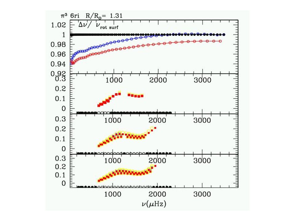
Non uniform rotation detectable with Corot ? Uniform versus differential (depth) moderate rotation Hz) diff nlm - unif nlm l = 1 modes m = 0, +1 from JC Suarez 04 Surface v ~ 100 km/s core/ surf ~ 2 diff nlm - unif nlm radial order n differences > 1 Hz
 moderate rotation Hz) diff nlm - unif nlm l = 1 modes m = 0, +1 from JC Suarez 04 Surface v ~ 100 km/s core/ surf ~ 2 diff nlm - unif nlm radial order n differences > 1 Hz.")
55
FGK stars (solar like oscillators) External convective zone and rotation : dynamo and J loss : spin down from the surface ie redistribution of ang. mom and chemicals Ex. HD 171488 (G0, 30 Myr) ~ 20 sol (Strassmeier et al 2003) --> slow rotators but … black dots v in i > 12 km/s open dots v sin i < 12 km/s v sin i measurements
 ~ 20 sol (Strassmeier et al 2003) --> slow rotators but … black dots v in i > 12 km/s open dots v sin i < 12 km/s v sin i measurements.")
56
Solar like oscillators : slow rotators Splitting large enough to be detected not yet the splittings ! Seismic data from ground: First seismic models: Cen, Boo, Procyon Slow rotators then classical techniques with linear splittings: High frequency p-modes probe external layer rotation

57
Rotation forward and inversion possible for high enough, evolved enough solar like oscillator stars Mixed modes : a few indeed excited and detectable Boo type) access central rotation values but requires knowledge of a model close to the reality : seismic model 1.55 M sol with Corot estimated performances from Lochard et al 04 forward
 access central rotation values but requires knowledge of a model close to the reality : seismic model 1.55 M sol with Corot estimated performances from Lochard et al 04 forward")
58
FGK stars : slow rotators but excited modes = high frequency modes ie small inertia, more sensitive to surface properties and rotation more efficient in surface small separation a - b affected by degeneracy then echelle diagram affected is used for mode (l) identification then not affected (m=0 only) But with m components : a mess !!! FGK From Lochard et al 2004 l=2 l=0 l=3 l=1 Black dots =0 Open dots = 20, 30, 50 km/s 20km/s 30km/s 50 km/s

59
To built a seimic model, fit the small separation l a =3, l b =1 modes z no rot rot Small separation la,n - lb,n-1 ~1.2 Hz rot no rot from Lochard et al 04 1 Hz ~> 1Gy

61
l=1,l=3 small separation polluted by rotation (65 km/s) Small separation free of rotation pollution recovered Small separation with no rotation 1.54 M sol
 Small separation free of rotation pollution recovered Small separation with no rotation 1.54 M sol")
62
V n = (r) (P rot -P norot ) y n dr eigenmode pressure Vn is a measurable seismic quantity and can be inverted for the distorted structure With a little extra work: Another quantity can be measurable with mixed modes: S = (r) ( rot - norot ) y n dr density --> Strength of baroclinicity grad P ^ grad Get for free!:
 (P rot -P norot ) y n dr eigenmode pressure Vn is a measurable seismic quantity and can be inverted for the distorted structure With a little extra work: Another quantity can be measurable with mixed modes: S = (r) ( rot - norot ) y n dr density --> Strength of baroclinicity grad P ^ grad Get for free!:")
63
Summary : with seismology what we really want is to detect and localize grad Fast rotation = oblateness, baroclinic, shellular assumption ? Much better if we also have: * surface P rot or a relation between P rot and stellar parameters * Seismic model : (is wanted by itself and wanted for rotation determination) better use slow rotators if possible otherwise must remove pollution by rotation AND COROT data! Must use all what we have : seismic and nonseismic info complementary forward and inverse info
 better use slow rotators if possible otherwise must remove pollution by rotation AND COROT data. Must use all what we have : seismic and nonseismic info complementary forward and inverse info.")
64
Further work before june 2006: visibility, mode identification versus rotation validity of perturbation techniques, 2D calculations initial conditions: rotation profile of slow rotators depends on its history latitudinal dependence (observations from ground already) warning!: probably not possible to consider only by itself: relation with B, activity, convection ….
 warning!: probably not possible to consider only by itself: relation with B, activity, convection ….")
65
FIN

66
Rotating convective core of A stars 3 D simulations (Browning et al 2004) 2 M sol ; rotation 1/10 to 4 times sol Rotating convective core is prolate Rotating convective is nonhomogeneous
 2 M sol ; rotation 1/10 to 4 times sol Rotating convective core is prolate Rotating convective is nonhomogeneous")
67
Overshoot from a rotating convective core 3D simulations: Extension of overshoot modified by rotation Rotation increases --> larger mixed region Heat (enthalpy) flux
 flux")
68
Long oscillation periods: g modes Asymptotics yields radial order Slow rotators Seismic models are built (non unique) Next : use mode excitation (nonadiabatic) information but must take into account effects of small (Dintrans, Rieutord, 2000) D Dor (Moya et al. 2004)
.")
69
Advantages: no external convective zone, mode identification more fiable; slow rotator: rotation as an advantage and not a problem; mixed p-g modes ; splitting << large sep/2 Inconvenients: long periods : 3h-8h The Cepheid HD 129929 : (Dupret et al 04; Aerts et al 04) Lot of effort ! : multisite observations + multitechniques then frequencies + location in HR diagram + mode identification (l degree) + nonadiabatic (n order) then Seismic models can be built
 + nonadiabatic (n order) then Seismic models can be built.")
70
From MA Dupret A triplet l=1 and some l=2 components yield : d ov = 0.1 +_ 0.05 = core + (x-1) 1 =.0071334 - 0.0185619 (x-1) c/d ; x=r/R --> Core rotates faster than envelope (surface 2 km/s) Rotation kernels Vaissala frequency x=r/R CoreSurface Vaissala pulsation : buoyancy restoring force/unit mass p modes g modes
 1 = (x-1) c/d ; x=r/R --> Core rotates faster than envelope (surface 2 km/s) Rotation kernels Vaissala frequency x=r/R CoreSurface Vaissala pulsation : buoyancy restoring force/unit mass p modes g modes")
71
ie linked to distorted structure quantities

72
Second order perturbation : a b a obs b obs Add near degenerary

73
PMS: protostars rotate fast. Interaction with disk ? Spin down, spin up phases ? End of life: - mass loss mechanisms ? - rotation of remnants WD ? - asymmetric nebulae ? - role of rotation of pre-supernova central stars ? What ? Rotation and related processes PMS to compact objects Massive stars : WR stages, yields Small and intermediate and mass stars Small to massive stars

74
from M. Rieutord Aussois 04

Similar presentations


>")


 G. Fontaine and P.>")


>")


Département de physique, Université.>")