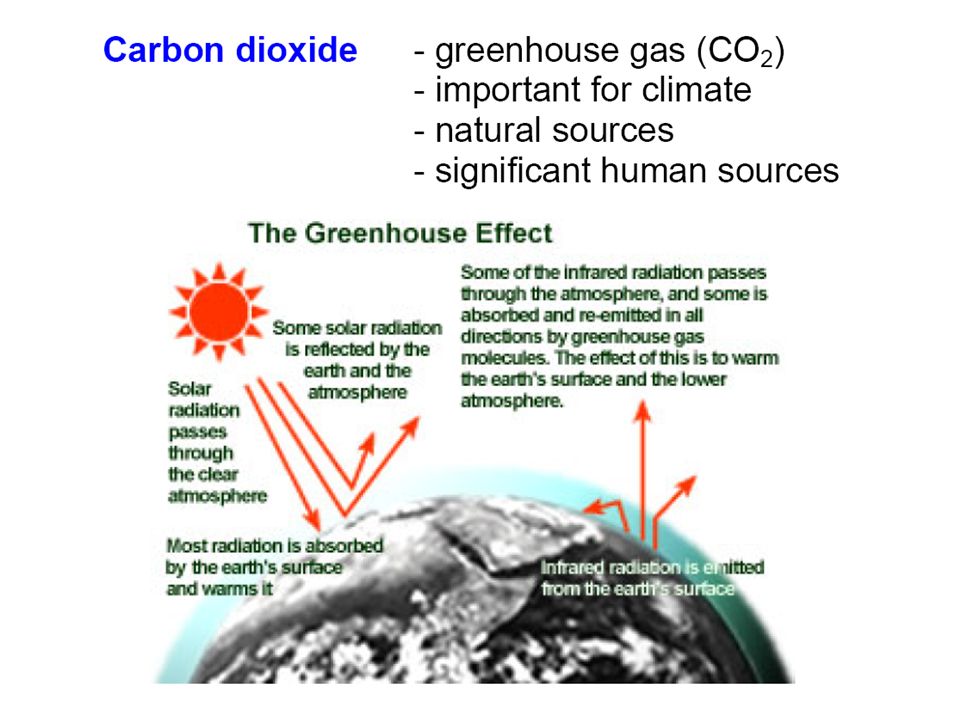
1. Greenhouse Gases Permanent gases Variable gases GHGs Ozone Suspended particles 30 o cooler w/o GHGs! This file forked from 9 Sep 09 Climate Chage Compresed

2. Image shows the emission from the infrared portion of the solar spectrum. Bright areas represent cold high cloud tops. Dark areas represent warm ground and ocean surfaces. These images are color coded to enhance high cloud tops http://weather.unisys.com/satellit e/infrared_enh.html Surface Emission

3. John Dalton Constant components (proportions remain the same over time and location) Nitrogen (N 2 )78.08% Oxygen (O 2 )20.95% Argon (Ar)0.93% Neon, Helium, Krypton0.0001% Variable components (amounts vary over time and location) Carbon dioxide (CO 2 )0.038% Water vapor (H 2 0)0-4% Methane (CH 4 )trace Sulfur dioxide (SO 2 )trace Ozone (O 3 )trace Nitrogen oxides (NO, NO 2 )trace The Atmosphere GHGs absorb heat emitted by the earth N 2 and O 2 have little effect on weather and atmospheric processes

4. http://www.indiana.edu/~geog109/topics/01_atmosphere/atmosphere.pdf Proportions

5. Water Vapor Image from observatory.ph

6. Water Vapor: Latent Heat Evaporative coolers take advantage of liquid to gas transition Clouds & precipitation: incoming (solar) radiation and outgoing longwave radiation

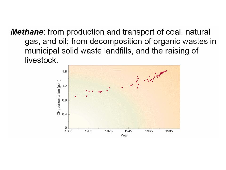
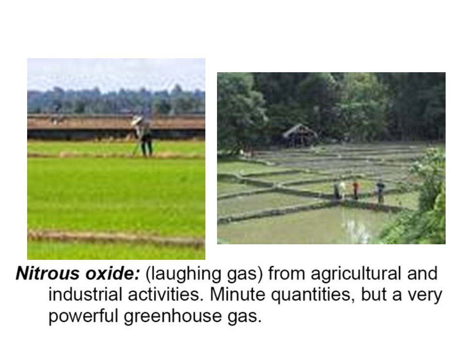
10. Industrial Byproducts

11. Equivalent CO 2

12. Solar Spectrum http://www.vicphysics.org/events/stav2005.html Energy f  c h f = E

13. Thermal Radiation “Blanket” http://www.te-software.co.nz/blog/augie_auer.htm

14. Energy: 50,038 kt Energy industries15,509 Residential 4,358 Industries 9,496 Agriculture 1,190 Transport 15,889 Commercial 3,369 Fugitive Emissions 227 TOTAL50,038

15. Industry: 10,711 kt Cement 4,771 Chemicals 99 Metals 4,334 Halocarbons 1,507 TOTAL10,711

16. Agriculture: 33,138 kt Rice 13,364 Livestock 10,497 Residue Burning 583 Soils 8,686 Grassland Burning 8 TOTAL 33,138

17. Waste: 9,198.3 kt Solid Waste 6,357.3 Domestic Wastewater 966.4 Industrial Wastewater 920.4 Human Sewage 954.2 TOTAL 9,198.3

18. LUCF: -127 kt Change in Biomass Biomass Growth -110,381 Roundwood/Fuelwood harvest 42,381 On-site burning28,866 Off-site burning 6,555 Decay 32,774 TOTAL -127

19. National carbon dioxide (CO2) emissions per capita. Shows various countries and their levels of CO2 emissions per capita. Also indicates the difference from high income to low income nations on CO2 output. Central to any study of climate change is the development of an emissions inventory that identifies and quantifies a country’s primary anthropogenic sources and sinks of greenhouse gas. Emissions are not usually monitored directly, but are generally estimated using models. Some emissions can be calculated with only limited accuracy. Emissions from energy and industrial processes are the most reliable (using energy consumption statistics and industrial point sources). Some agricultural emissions, such as methane and nitrous oxide carry major uncertainties because they are generated through biological processes that can be quite variable. Per Capita Emission UNEP/GRID-Arendal, National carbon dioxide (CO2) emissions per capita, UNEP/GRID-Arendal Maps and Graphics Library, http://maps.grida.no/go/graphic/national_carbon_dioxide_co2_emissions_per_capitahttp://maps.grida.no/go/graphic/national_carbon_dioxide_co2_emissions_per_capita

20. http://www.carbonplanet.com/country_emissions Emissions by Country

21. http://www.esrl.noaa.gov/gmd/ccgg/trends/ The graph shows recent monthly mean carbon dioxide measured at Mauna Loa Observatory, Hawaii. The last four complete years of the Mauna Loa CO2 record plus the current year are shown. Data are reported as a dry mole fraction defined as the number of molecules of carbon dioxide divided by the number of molecules of dry air, multiplied by one million (ppm) Mauna Loa The dashed red line with diamond symbols represents the monthly mean values, centered on the middle of each month. The black line with the square symbols represents the same, after correction for the average seasonal cycle. The latter is determined as a moving average of five adjacent seasonal cycles centered on the month to be corrected, except for the first and last two and one- half years of the record, where the seasonal cycle has been averaged over the first and last five years, respectively. The Mauna Loa data are being obtained at an altitude of 3400 m in the northern subtropics, and may not be the same as the globally averaged CO2 concentration at the surface. globally averaged CO2 concentration at the surface CO 2 Annual Cycle Biospheric respiration in winter Photosynthesis in summer

22. http://www.esrl.noaa.gov/gmd/ccgg/trends/ The graph shows recent monthly mean carbon dioxide measured at Mauna Loa Observatory, Hawaii. The last four complete years of the Mauna Loa CO2 record plus the current year are shown. Data are reported as a dry mole fraction defined as the number of molecules of carbon dioxide divided by the number of molecules of dry air, multiplied by one million (ppm) The dashed red line with diamond symbols represents the monthly mean values, centered on the middle of each month. The black line with the square symbols represents the same, after correction for the average seasonal cycle. The latter is determined as a moving average of five adjacent seasonal cycles centered on the month to be corrected, except for the first and last two and one-half years of the record, where the seasonal cycle has been averaged over the first and last five years, respectively. The Mauna Loa data are being obtained at an altitude of 3400 m in the northern subtropics, and may not be the same as the globally averaged CO2 concentration at the surface.globally averaged CO2 concentration at the surface CO 2 Annual Cycle Biospheric respiration in winter Photosynthesis in summer

23. Carbon Cycle Aquatic and Terrestrial Carbon Cycles Carbon = Life; Carbon = Energy

24. carbon dioxide + water + solar energy  glucose + oxygen 6 CO 2 + 6 H 2 O + E solar  C 6 H 12 O 6 + 6O 2 Carbon dioxide to oxygen Chlorophyll molecules are specifically arranged in and around pigment protein complexes called photosystems which are embedded in the thylakoid membranes of chloroplasts.photosystemsthylakoid chloroplasts http://en.wikipedia.org/wiki/Chlorophyll Photosynthesis

25. http://www.chm.bris.ac.uk/motm/chlorophyll/chlorophyll_h.htm Chlorophyll

26. Animals-Consumers + Oxygen + Glucose  CO2 + Water (respiration) C 6 H 12 O 6 + 6 O 2 --> 6 CO 2 + 6 H 2 O Respiration

27. Climate Change Model http://ccl.northwestern.edu/netlogo/models/ClimateChange

28. When organic matter accumulates faster than decomposition processes Terrestrial Carbon Cycle

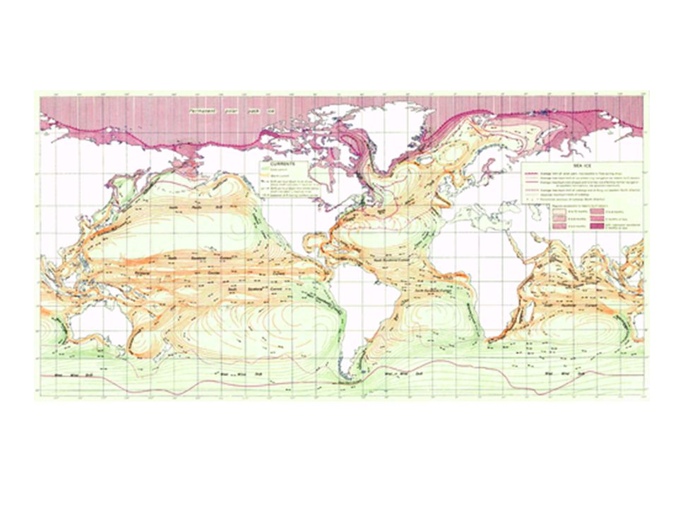
29. Aquatic Carbon Cycle Rocks and sediments http://www.lenntech.com/carbon-cycle.htm Warming of ocean

30. Melting permafrost peatlands at Noyabrsk, Western Siberia. http://www.terranature.org/methaneSiberia.htm A study published in the September 7th issue (2006) of Nature authored by Katey Walter of the University of Alaska, and Jeff Chanton of Florida State University reports that greenhouse gas is escaping into the atmosphere at a frightening rate. CO 2 “locked in” the Permafrost

31. Within the framework of the joint European Greenland Ice Core Project (GRIP) a 3029 m long ice core was drilled in Central Greenland from 1989 to 1992 at 72 o 35' N, 37 o 38' W. Polar ice cores contain a record of the past atmosphere - temperature, precipitation, gas content, chemical composition, and other properties. The objective of the GRIP effort was to reveal the broad spectrum of information on past environmental, and particularly climatic, changes that are stored in the ice. This information will help investigators understand the major mechanisms of the earth and man's potential impact. K. Makinson The Greenland Ice Core Project (GRIP) http://www.ncdc.noaa.gov/paleo/icecore/greenland/s ummit/document / Studies of isotopes and various atmospheric constituents in the core have revealed a detailed record of climatic variations reaching more than 100,000 years back in time. The results indicate that Holocene climate has been remarkably stable and have confirmed the occurrence of rapid climatic variation during the last ice age (the Wisconsin). Climatic instability observed in the core part believed to date from the Eemian interglacial has not been confirmed by other climate records

32. Antarctic Ice Cores

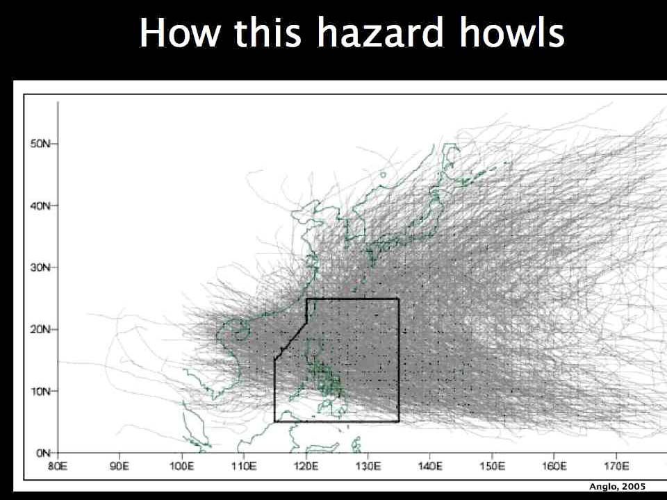
33. Temperature Rise Changing typhoon trajectory and intensity Sea Level Rise Perturbed Ocean Currents Extreme Events (stronger typhoons, heat waves) Coral Bleaching Expansion and extension of tropical diseases Impact

34. http://nsidc.org/data/iceshelves_images/ Arctic

35. Temperature increases in the Arctic due to climate change, 2090 (NCAR-CCM3, SRES A2 experiment). Climate change, due to increased concentrations of greenhouse gases in the atmosphere, has lead to increased temperatures and large scale changes in the Arctic. The Arctic sea ice is decreasing, permafrost thawing and the glaciers and ice sheets are shrinking. Temperature increases in the Arctic due to climate change, 2090 (NCAR-CCM3, SRES A2 experiment). (2008). In UNEP/GRID-Arendal Maps and Graphics Library.

36. Projected temperature increases due to climate change. Some of the ice shelves of the Antarctic peninsula have split up and started moving more rapidly, but the analyses of the Antarctic ice sheet are inconclusive. The projected climate situation in 2090 are presented in this figure, the temperatures are annual values from the NCAR-CCM3 model, ensemble averages 1-5 for the SRES A2 experiment. UNEP/GRID-Arendal, Temperature increases in the Antarctic due to climate change, 2090 (NCAR-CCM3, SRES A2 experiment), UNEP/GRID-Arendal Maps and Graphics Library, http://maps.grida.no/go/graphic/temperature-increases-in- the-antarctic-due-to-climate-change-2090-ncar-ccm3-sres-a2-experimenthttp://maps.grida.no/go/graphic/temperature-increases-in- the-antarctic-due-to-climate-change-2090-ncar-ccm3-sres-a2-experiment Antarctic

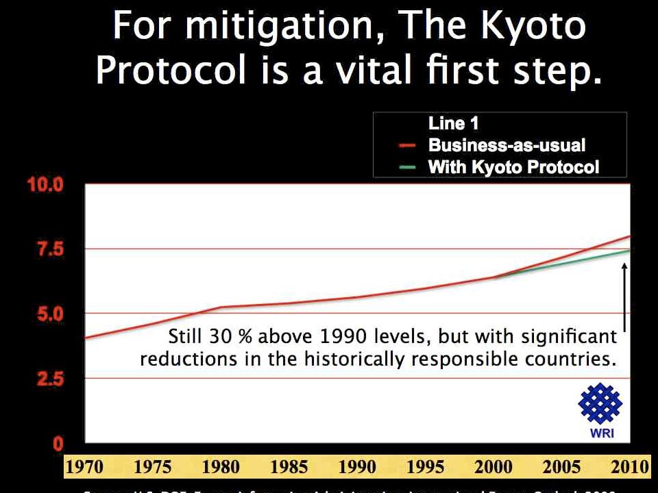
39. Sea Levels http://www.grida.no/climate/vital/19.htm

40. It is likely that much of the rise in sea level has been related to the concurrent rise in global temperature over the last 100 years. On this time scale, the warming and the consequent thermal expansion of the oceans may account for about 2-7 cm of the observed sea level rise, while the observed retreat of glaciers and ice caps may account for about 2-5 cm. Other factors are more difficult to quantify. The rate of observed sea level rise suggests that there has been a net positive contribution from the huge ice sheets of Greenland and Antarctica, but observations of the ice sheets do not yet allow meaningful quantitative estimates of their separate contributions. The ice sheets remain a major source of uncertainty in accounting for past changes in sea level because of insufficient data about these ice sheets over the last 100 years http://www.grida.no/climate/vital/19.htm Sea Levels Over the last 100 years, the global sea level has risen by about 10 to 25 cm. Sea level change is difficult to measure. Relative sea level changes have been derived mainly from tide-gauge data. In the conventional tide-gauge system, the sea level is measured relative to a land-based tide-gauge benchmark. The major problem is that the land experiences vertical movements (e.g. from isostatic effects, neotectonism, and sedimentation), and these get incorporated into the measurements. However, improved methods of filtering out the effects of long-term vertical land movements, as well as a greater reliance on the longest tide-gauge records for estimating trends, have provided greater confidence that the volume of ocean water has indeed been increasing, causing the sea level to rise within the given range. http://www.bodc.ac.uk/data/online_delivery/ntslf/

41. Extreme Storms It formed over the Bahamas on August 23, 2005, and crossed southern Florida as a moderate Category 1 hurricane, causing some deaths and flooding there, before strengthening rapidly in the Gulf of Mexico and becoming one of the strongest hurricanes on record while at sea. The storm weakened before making its second and third landfalls as a Category 3 storm on the morning of August 29 in southeast Louisiana and at the Louisiana/Mississippi state line, respectively.BahamasAugust 23 2005FloridaGulf of MexicoAugust 29 Hurricane Katrina was the costliest and one of the five deadliest hurricanes in the history of the United States.[3] It was the sixth- strongest Atlantic hurricane ever recorded and the third-strongest hurricane on record that made landfall in the United States. Katrina formed on August 23 during the 2005 Atlantic hurricane season and caused devastation along much of the north-central Gulf Coast. The most severe loss of life and property damage occurred in New Orleans, Louisiana, which flooded as the levee system catastrophically failed, in many cases hours after the storm had moved inland.[4] The hurricane caused severe destruction across the entire Mississippi coast and into Alabama, as far as 100 miles (160 km) from the storm's center. In the 2005 Atlantic season, Katrina was the eleventh tropical storm, fifth hurricane, third major hurricane, and second Category 5 hurricane. hurricanesUnited States[3]AtlantichurricanelandfallAugust 232005 Atlantic hurricane seasonGulf Coastloss of life and property damageNew OrleansLouisianalevee[4]Mississippimajor hurricaneCategory 5 hurricane http://en.wikipedia.org/wiki/Hurricane_Katrina

42. Simulated Increase of Hurricane Intensities in a CO 2 -Warmed Climate Thomas R. Knutson, * Robert E. Tuleya, Yoshio Kurihara Hurricanes can inflict catastrophic property damage and loss of human life. Thus, it is important to determine how the character of these powerful storms could change in response to greenhouse gas- induced global warming. The impact of climate warming on hurricane intensities was investigated with a regional, high-resolution, hurricane prediction model. In a case study, 51 western Pacific storm cases under present-day climate conditions were compared with 51 storm cases under high-CO 2 conditions. More idealized experiments were also performed. The large-scale initial conditions were derived from a global climate model. For a sea surface temperature warming of about 2.2°C, the simulations yielded hurricanes that were more intense by 3 to 7 meters per second (5 to 12 percent) for wind speed and 7 to 20 millibars for central surface pressure. Geophysical Fluid Dynamics Laboratory/National Oceanic and Atmospheric Administration, Post Office Box 308, Princeton, NJ 08542, USA. * To whom correspondence should be addressed. E-mail: tk@gfdl.govtk@gfdl.gov Science 13 February 1998: Vol. 279. no. 5353, pp. 1018 - 1021 DOI: 10.1126/science.279.5353.1018

44. Corals + elevated temp., high light intensities, pollutants…..

45. http://en.wikipedia.org/wiki/File:Bethlehem_Steel_Pennellb.jpg

47. http://unfccc.int/meetings/cop_14/items/4481.php Ban Ki-Moon, UN Secretary General