Download presentation
Presentation is loading. Please wait.

1
Switch off your Mobiles Phones or Change Profile to Silent Mode

2
Relational Algebra and Physical Database Design

3
Relational Algebra

4
Topics Definition of Algebra Algebra Operators and Syntax Application of Algebraic Operators Sample Queries

5
Relational Algebra Relational Algebra is a set of operations which can be applied to a relational database in order to manipulate and access data contained in relations (tables) These set of operations fall into two categories: Traditional set operations union, intersection, product and difference. Special relational operations restriction, projection, join and division.

6
Definition of Algebra

7
Relational Algebra Operators RESTRICT Extracts specified tuples from a specified relation (i.e. restricts the specified relation to just those tuples that satisfy a specified condition). PROJECT Extracts specified attributes from a specified relation.
. PROJECT Extracts specified attributes from a specified relation..")
8
Relational Algebra Operators PRODUCT Builds a relation from two specified relations consisting of all possible combinations of tuples, one from each of the two relations. UNION Builds a relation consisting of all tuples appearing in either or both of two specified relations.

9
Relational Algebra Operators INTERSECTION Builds a relation consisting of all tuples appearing in both of two specified relations. DIFFERENCE Builds a relation consisting of all tuples appearing in the first and not the second of two specified relations

10
Relational Algebra Operators JOIN Builds a relation from two specified relations consisting of all possible combinations of tuples, one from each of the relations, such that the two tuples contributing to any given combination satisfy some specified condition.

11
Relational Algebra Operators DIVIDE Takes two relations, one binary and one unary, and builds a relation consisting of all values of one attribute of the binary relation that match all values in the unary relation.

12
Relational Algebra Syntax RESTRICT relation-name-1 WHERE condition [GIVING relation-name-2] PROJECT relation-name-1 OVER attribute-list [GIVING relation-name-2] JOIN relation-name-1 AND relation- name-2 [OVER common-attribute-list] [GIVING relation-name-3]
![Relational Algebra Syntax RESTRICT relation-name-1 WHERE condition [GIVING relation-name-2] PROJECT relation-name-1 OVER attribute-list [GIVING relation-name-2] JOIN relation-name-1 AND relation- name-2 [OVER common-attribute-list] [GIVING relation-name-3]](http://images.slideplayer.com/26/8602219/slides/slide_12.jpg "Relational Algebra Syntax RESTRICT relation-name-1 WHERE condition [GIVING relation-name-2] PROJECT relation-name-1 OVER attribute-list [GIVING relation-name-2] JOIN relation-name-1 AND relation- name-2 [OVER common-attribute-list] [GIVING relation-name-3]")
13
Relational Algebra Syntax DIVIDE dividend-relation-name BY divisor-relation-name [OVER common- attribute-list] [GIVING relation-name-1] relation-name-1 UNION relation-name-2 [GIVING relation-name-3] relation-name-1 DIFFERENCE relation- name-2 [GIVING relation-name-3] relation-name-1 INTERSECT relation- name-2 [GIVING relation-name-3]
![Relational Algebra Syntax DIVIDE dividend-relation-name BY divisor-relation-name [OVER common- attribute-list] [GIVING relation-name-1] relation-name-1 UNION relation-name-2 [GIVING relation-name-3] relation-name-1 DIFFERENCE relation- name-2 [GIVING relation-name-3] relation-name-1 INTERSECT relation- name-2 [GIVING relation-name-3]](http://images.slideplayer.com/26/8602219/slides/slide_13.jpg "Relational Algebra Syntax DIVIDE dividend-relation-name BY divisor-relation-name [OVER common- attribute-list] [GIVING relation-name-1] relation-name-1 UNION relation-name-2 [GIVING relation-name-3] relation-name-1 DIFFERENCE relation- name-2 [GIVING relation-name-3] relation-name-1 INTERSECT relation- name-2 [GIVING relation-name-3]")
14
Student Marks Example

15
Relational Algebra Closure Property Use of relational algebra operators on existing relations (tables) produces new valid output relation. Each output relation can then be safely used in a subsequent operation.

16
Union Operator UNION combines all rows from two relations, excluding duplicate rows. The relations must have the same attribute characteristics (the columns and domains must be identical) to be used in the UNION. Union Compatibility Iff the two input relations have identical headings
 to be used in the UNION. Union Compatibility Iff the two input relations have identical headings.")
17
Union Operator 3 rd Year Students UNION 2 nd Year Students

18
Intersect Operator INTERSECT yields only the rows that appear in both relations. The relations must be union-compatible to yield valid results. For example, you cannot use INTERSECT if one of the attributes is numeric and one is character-based.

19
Intersect Operator

20
Difference Operator DIFFERENCE yields all rows in one relation that are not found in the other relation; that is, it subtracts one relation from the other. The relations must be union-compatible to yield valid results

21
Difference Operator

22
Restrict Operator RESTRICT, also known as SELECT, yields values for all rows found in a relation that satisfy a given condition. RESTRICT can be used to list all of the row values, or it can yield only those row values that match a specified criterion. In other words, RESTRICT yields a horizontal subset of a relation.

23
Restrict Operator

24
Project Operator PROJECT yields all values for selected attributes. In other words, PROJECT yields a vertical subset of a relation.

25
Project Operator

26
Product Compatibility Iff the two input relations have disjoint headings.

27
Product Operator

29
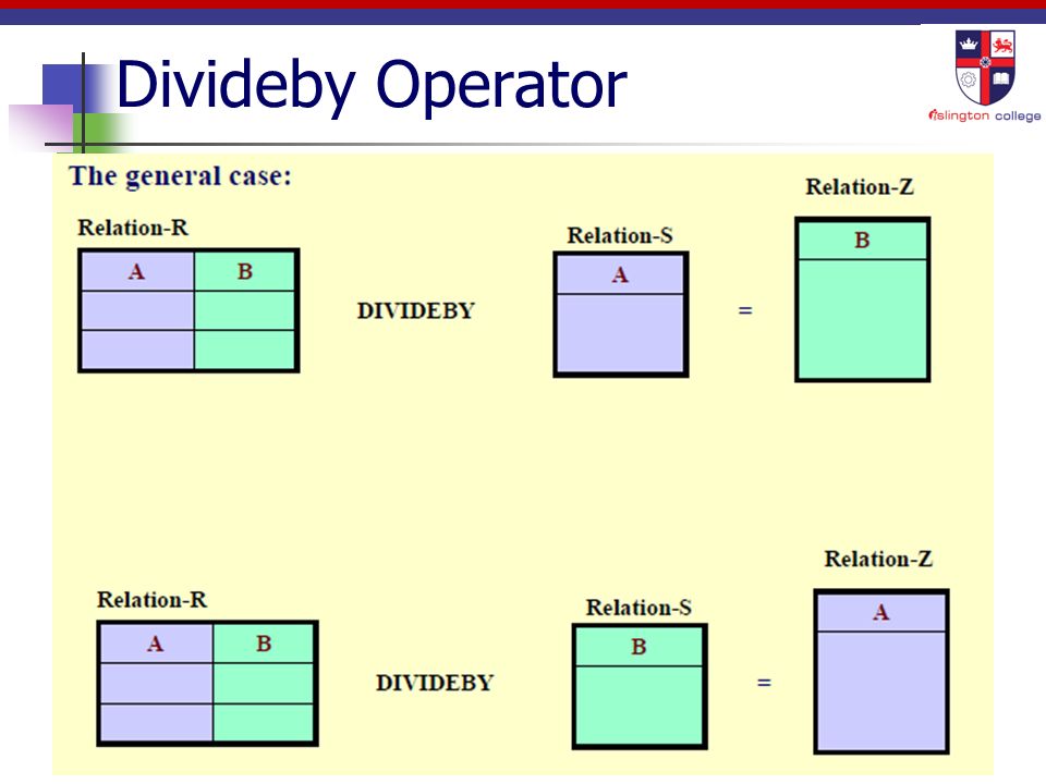
Divideby Operator

32
Join Operator JOIN allows information to be combined from two or more relations. JOIN allows the use of independent relations linked by common attributes. Different types of JOIN: theta join where join condition is any of =, >, =, <= equi join where join condition is = natural join where join condition is = but only one join column is presented in result

33
Join Operator

34
Relational Algebra and SQL We can identify differences between Relational Algebra and SQL SQLRelational Algebra CommercialNot Implemented DeclarativeProcedural Optimised by Query OptimiserSequence of Operations

35
Physical Database Design

36
Objective is to select physical representations for each relation such that the database has following properties: data may be accessed with acceptable speed database does not use up too much of computer’s store database is reasonably resilient to catastrophes.

37
Physical Database Design Physical design decisions should be based on following: logical database design. quantities and volatility of data. ways in which the data is used. costs associated with storing and accessing data.

38
Physical Database Design Physical database design typically proceeds as follows: an initial design is generated based on anticipated processing. initial design is tested and data manipulations are ‘bench-marked’. modifications can be made is necessary, bottlenecks are identified and rectified. monitoring and continued, appropriate modifications.

39
Representation of Relations Relations are usually represented as computer files in which a record represents a tuple/row.

40
File Handling Files are handled by the operating system, and so RDBMSs usually sit on top of the operating system’s file manager.

41
File Structure Techniques Heap files and Serial search Constructed as a list of pages - when a new record is inserted it is placed in the last page of the file. Advantages fast record insertion economic use of store Disadvantages serial search is slow reclamation of space not possible

42
File Structure Techniques Access Keys When accessing data, a search condition is usually applied to restrict the rows retrieved: SELECT * FROM PART WHERE part_no = ‘P1’ AND price > 22; Part_no is tighter key than price, which is a looser key

43
File Structure Techniques Sorted Files Speed of some retrievals may be improved by ensuring that file records are stored in some specific order. Advantages easy to define access key facilitates the binary search Disadvantages maintenance of the sequence

44
File Structure Techniques Sorted Files - using Binary Search Binary search is technique of repeatedly halving a file and searching the half in which searched record is stored. SELECT * FROM PART WHERE part_no = ‘P9’

45
File Structure Techniques Hash (random) files Hashing is process of calculating location of a record from an access key value. Home address is computed address (page address) Hash key another name for the access key used Hashing function calculation used to compute home address
 Hash key another name for the access key used Hashing function calculation used to compute home address.")
46
File Structure Techniques Hash (random) files
 files")
47
File Structure Techniques Hash (random) files – an example:
 files – an example:")
48
File Structure Techniques Hash (random) files Advantages potentially very fast Disadvantages collision at home address
 files Advantages potentially very fast Disadvantages collision at home address")
49
Normalisation Normalisation is a technique for deciding which attributes belong together in a relation. Result of normalisation is a logical database design that is structurally consistent and has minimal redundancy. Sometimes argued that a normalised database design does not provide maximum processing efficiency.

50
Normalisation There may be circumstances where it may be necessary to accept the loss of some of the benefits of a fully normalised design in favor of performance. Should be considered only when it is estimated that the system will not be able to meet its performance requirements. Normalisation forces us to understand completely each attribute that has to be represented in the database.

51
Denormalisation Denormalisation refers to a refinement to relational schema such that the degree of normalisation for a modified relation is less than degree of at least one of the original relations. We also use the term more loosely to refer to situations where we combine two relations into one new relation, and new relation is still normalised but contains more nulls than the original relations.

52
Denormalisation Denormalisation is a set of techniques which may be applied to design to improve performance of queries. There are four techniques in denormalising duplicate data derived data surrogate keys vector data

53
Denormalisation Duplicate data Individual fields introduced redundantly to reduce number of records accessed.

54
Denormalisation Duplicate data Individual fields introduced redundantly to reduce number of records accessed.

55
Denormalisation Duplicate data Individual fields introduced redundantly to reduce number of records accessed.

56
Denormalisation Duplicate data Individual fields introduced redundantly to reduce number of records accessed.

57
Denormalisation Derived data: Summary or calculated fields introduced redundantly to reduce number of records involved in arithmetic.

58
Denormalisation Derived data: Summary or calculated fields introduced redundantly to reduce number of records involved in arithmetic.

59
Denormalisation Surrogate keys: Artificial keys introduced in place of inefficient key fields.

60
Denormalisation Vector data: Concept of multiple repeating fields reintroduced to group data in one record.

61
Denormalisation Relational theory will resolve a situation of storing 12 monthly account balances like this: BANK_ACC (account_no, name, address) ACC_BAL (account_no, month_no, balance) Vector data solution is: BANK_ACC (account_no, name, address, balance1, balance2,… ……, balance11, balance12)
 ACC_BAL (account_no, month_no, balance) Vector data solution is: BANK_ACC (account_no, name, address, balance1, balance2,… ……, balance11, balance12)")
62
Denormalisation Problem If you denormalise for performance, you do want to be sure that denormalisation is truly beneficial and that there is no better alternative. Denormalised tables will almost always be created by combining two or more normalised tables. rows will be longer each access will require more data transmission

63
Denormalisation Problem Denormalisation makes implementation more complex Denormalization often sacrifices flexibility Denormalization may speed up retrievals but it slows down updates. Data which is frequently updated should not be replicated without good reason.

64
When to Denormalise If performance is unsatisfactory and a relation has a low update rate and a very high query rate, denormalisation may be a viable option.

65
Any Questions?

Similar presentations