1. Supplementary PPT File for More detail explanation on SPSS Anova Results PY Cheng Nov., 2015

2. First Principle of Anova Test (Explained by Extreme perfect case)

3. Difference between the means is small relative to the sampling variation of scores within the treatments, we would not reject the null hypothesis of equal population means!

4. Difference between the sample variations is small relative to the difference between the two group means of scores, we would reject the null hypothesis of equal population means!

5. Three important assumptions for Anova test 1.Variables are independent with each other 2.Populations are normally distributed 3.Populations have equal variance Remarks : Anova is robust for deviation from normal distribution (i.e. not affected too much for moderate deviation!) However, it is rather sensitive to unequal variance, that can be handle better by Tukey’ Multiple Comparison Test with equal sample size!)

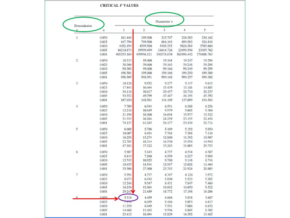
6. F Distribution and Usage of F value IF the 3 assumptions are fulfilled AND IF the samples are come from the SAME population i.e. with the same mean, a RATIO of ‘Between Group Error’ to ‘Within Group Error’ would form a ‘F Distribution’ determined by two degree of freedom.

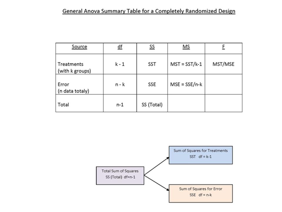
7. df1 = k-1 (Treatment with k groups) e.g. df1 = 2-1 = 1 df2 = n-k (Error by chance with n data totally) e.g. df2 = 10 – 2 = 8

10. Notice Anova is used for comparing 2 or > 2 group means (An Anova with 2 groups == a T Test with same var.) Null hypothesis: mean1 = mean2 =………..meank for k groups. Alternative hypothesis: at least two of the means are different When k > 2, We should not use a series of t-tests to substitute this Anova test, otherwise the chance of committing type I error would increase rapidly!

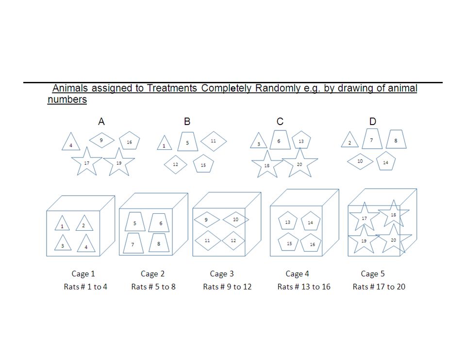
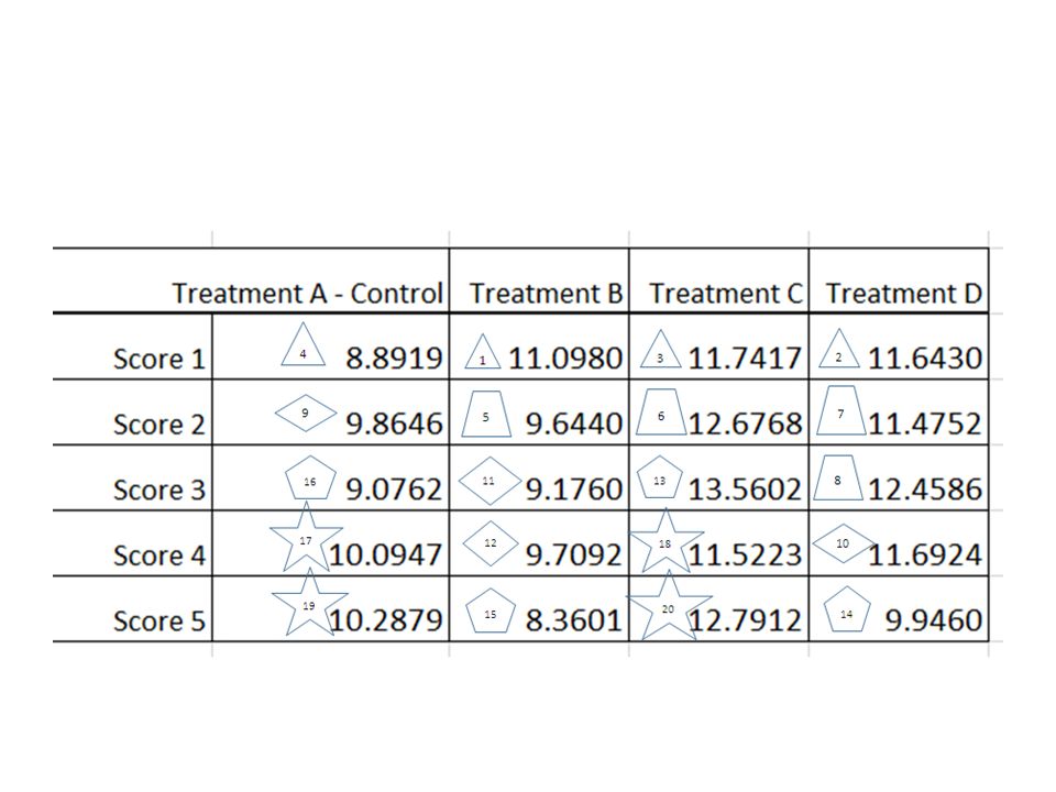
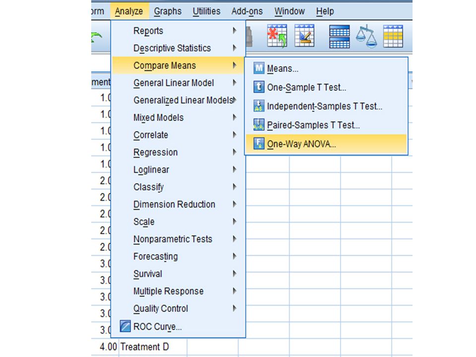
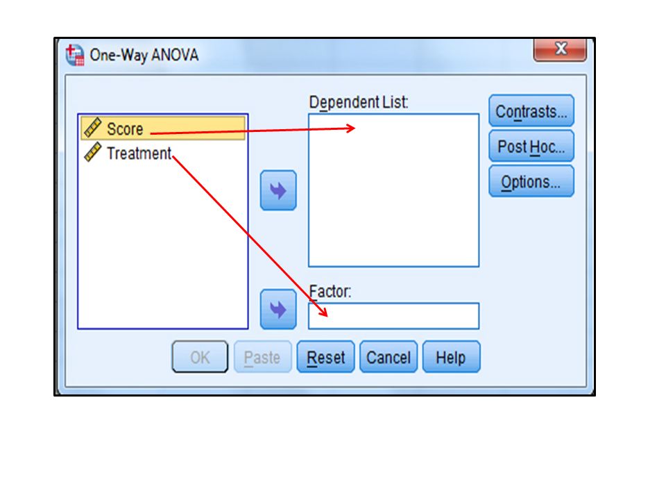
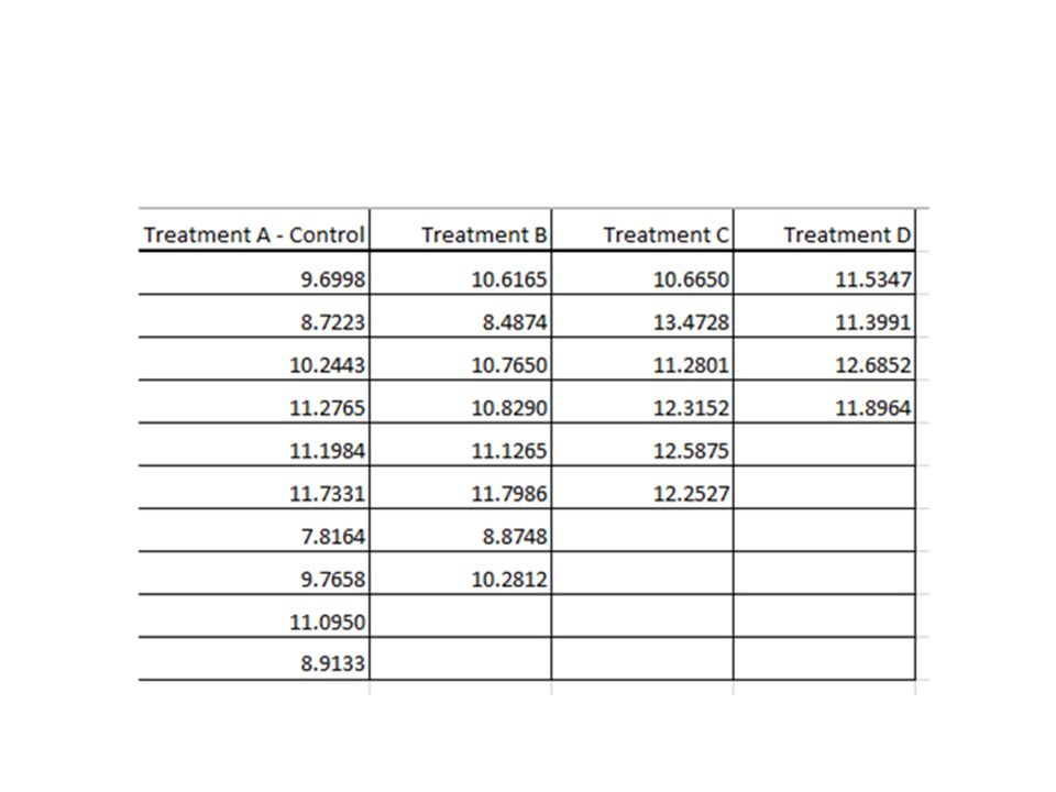
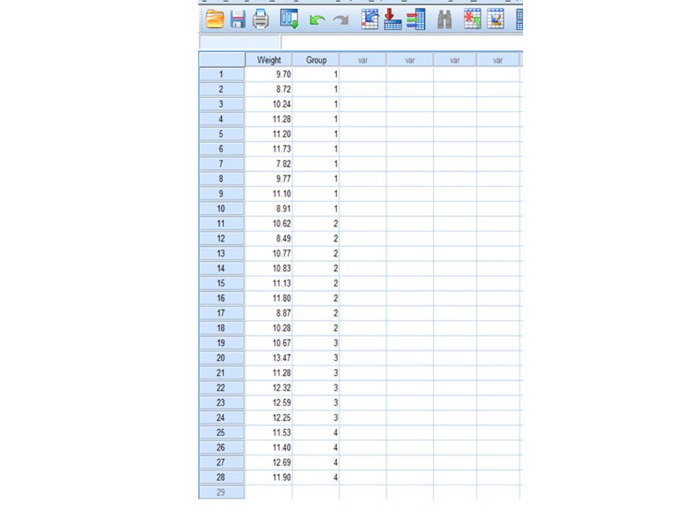
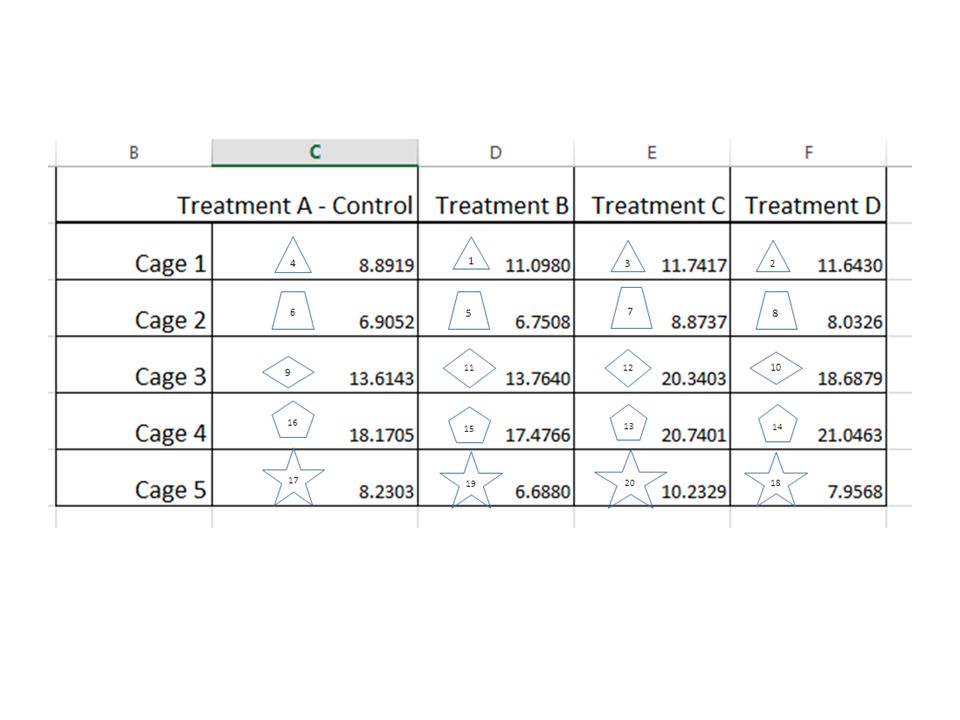
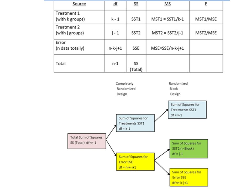
11. Completely Randomised Design Example 1.1.i (CRD with Equal Sample Size) 5 cages each with 4 rats were used for a ‘Completely Randomized Design’ Experiment. The 20 rats had been assigned to the treatments A (control), B, C and D totally randomly by e.g. blinded researcher drawing animal numbers, without concerning any cages boundaries! The response was a ‘score’ after the 4 ‘treatments’ e.g. a growth in body weight after a certain period of time. Please find any Significant Differences in this score caused by the four treatments :-

20. Not sign., equal variance assumption hold Sign < 0.05, at least 2 means diff. Where? See Multiple Comparisons!

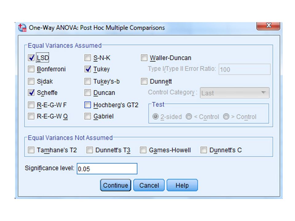
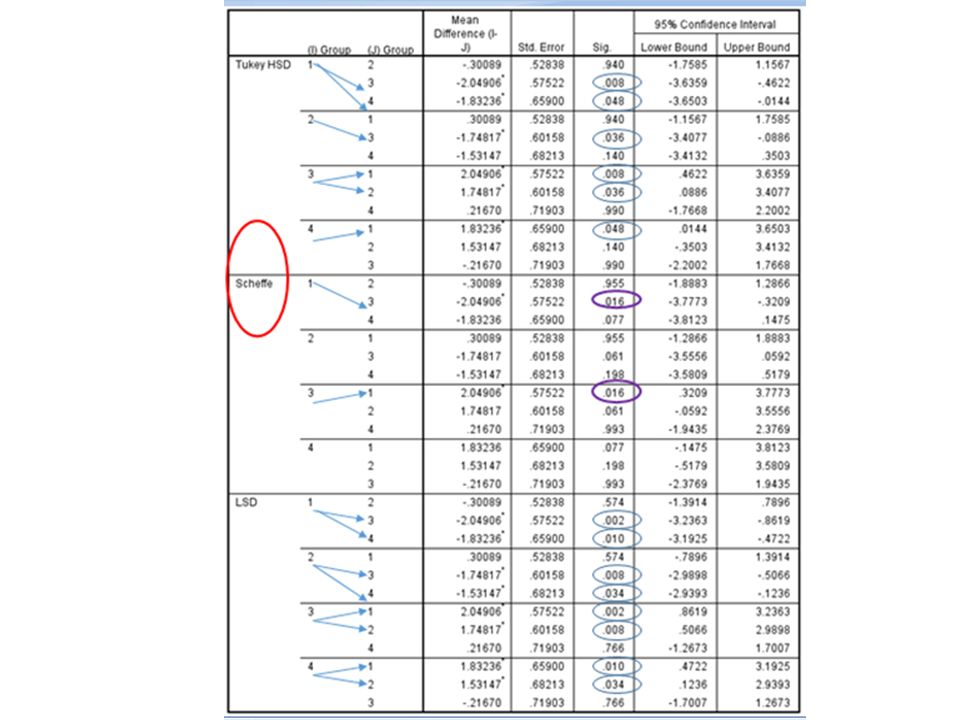
23. Tukey’s Test is most suitable in this equal sample size case – robust for deviation from equal variance assumption!! Groups 1 & 2 is really sign. different from Groups 3 & 4!

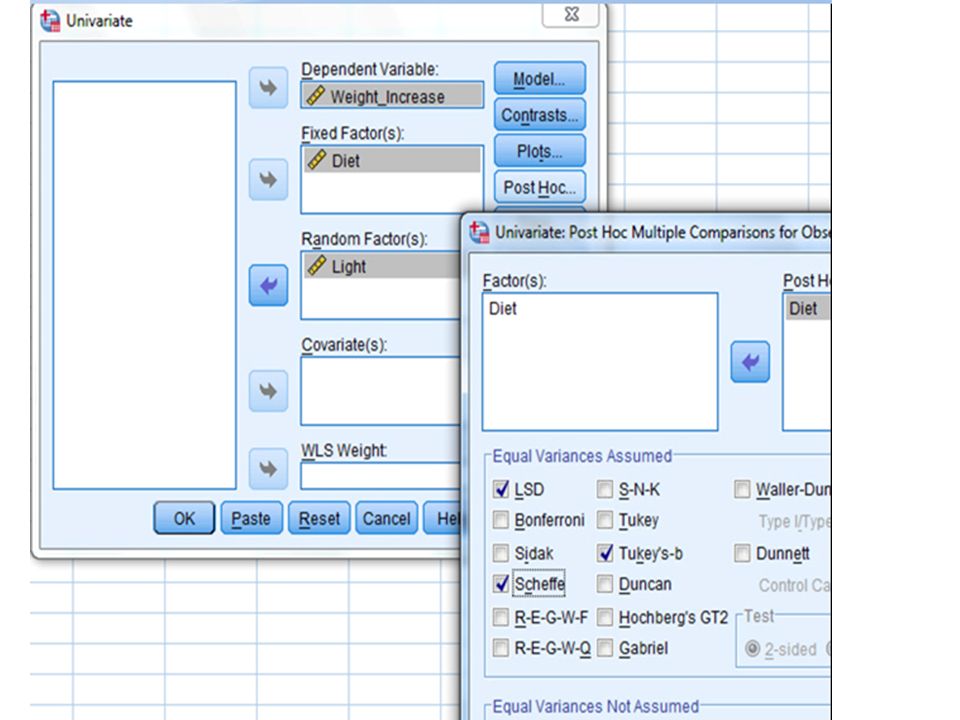
24. 1.1.ii Completely Randomised Design – Unequal Sample Size Under this situation the Tukey’s Test might not be suitable and the Scheffe’s Test should be used instead!

27. Not sign., equal variance assumption hold Sign < 0.05, at least 2 means diff. Where? See Multiple Comparisons!

29. Scheffe Test ‘Scheffe Test’ is customized for working on samples with unequal sample size, as in this example! The SPSS Scheffe Test results in only one inter-groups difference between Group 1 and Group 3. The ‘LSD’ Test is probably to too ‘loose’ and the ‘Tukey’ Test seems somewhere in between (Remark: SPSS uses ‘Tukey-Kramer’ test for unequal size case)!

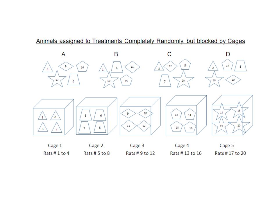
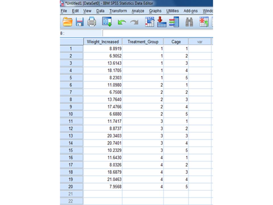
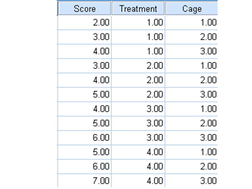
30. Completely Randomized Block Design Example 1.2.i – CRD, Blocked by Intention 5 cages each with 4 rats had been used for a Completely Randomized Block Design experiment. The 20 rats had been assigned to the treatments A (control), B, C and D. For each cage, one animal was drawn randomly for each treatment - it would allow getting rid of the effect of cages during data analysis! The response was a ‘score’ after the 4 ‘treatments’ e.g. a growth in body weight within a certain period of time.

33. The within-group error (points distances) might have been increased by the removing of confounding effect of different cages that can now be calculated under this block design!!

34. There seems to be obvious confounding effect (forming of groups) due to different cages!

36. Anova result without taking ‘cage’ into account. Not significant, cannot reject null hypothesis  all means equal!

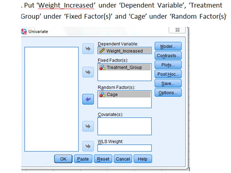
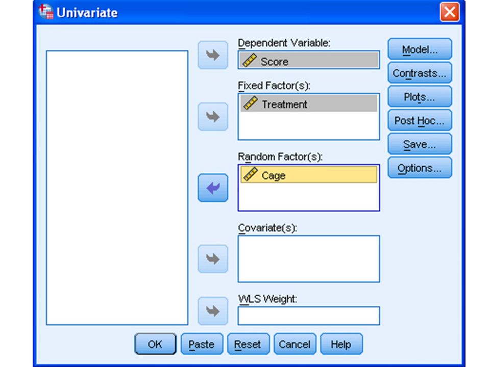
37. But the researcher suspected that this non- significance might due to the effect of different condition in different cages, so he made use of the ‘Block’ design with ‘Cage’ being a random factor to handle this effect. (Cannot do anything on this if not taking samples according to block design before experiment!)

41. Now we can find the ‘Sig.’ for ‘Treatment_Group’ = 0.03 < 0.05, meaning that the null hypothesis for equal means would be rejected. However, SPSS would not calculate the Post Hoc tests due to the sum and df of the error term both being zero, because of no replication of items. The having significance of the factor ‘Cage’( that ‘sig.’ =0.000 < 0.05) indicates that the blocking is correctly carried out.

42. Important Supplementary Documents for Interaction For any factorial designs with/without replication, there might be an interaction effect besides the main effects of factors. Document 1 on the attached CD offers a simple method for determining whether there is interaction or not! Please read P. 196 also! For designs without replication, either blocked or factorial, the residual sum of error might contain both interaction effect and random sampling error. Due to no replication, we generally cannot estimate how much error is due to interaction and how much error is due to sampling! So, we had better not to use this design if interaction is suspected among the main factors! However, we might still try to run a test on ‘Simple main effect’ to estimate whether the deviation from perfect case without interaction is purely due to chance or not! Please refer to Document 2 for this! !

43. Explanation by Extreme Case again The above issue might be explained by an extreme case again e.g. :-

44. Lines 100% parallel, either interaction nor random error, ALL ‘within Treatment group error’ is explained by belonging to which cage!! Treatment Score Cage 2 Cage 1 Cage 3

45. Lines 100% parallel, neither interaction nor random error, ALL ‘within case group error’ is explained by being under which treatment!! Cage Score Treatment A Treatment B Treatment C Treatment D

48. SPSS output for the extreme case Neither Interaction Nor Sampling Error Existing!

49. A real case would just be a deviation from this extreme case!! For example:- 1.83.44.45.6 3.84.86.2 4.55.25.87.3 2.5

50. Treatment Cage 1 Cage 2 Cage 3

51. Deviations from extreme case The arrows on the previous graph represent the deviations from the extreme case. They would be a mixture of:- Part 1) Interaction effect between Treatment and Case Part 2) Sampling error from the population Without replication, there is no way to calculate ‘Part 2’, we had better assume all of them is due to sampling error, and not to use this design if interaction is suspected between factors!!

54. Without replication, no sampling error at this level would exist! All assumed as random sampling error!

56. Blocked NOT by Intention

59. 0

60. Two Factors (aXb factorial) – Without Replication Without replication in each field of factor 1 and factor 2, the computer would not know about whether you are working for which of below: 1. Randomized design - blocked by intention 2. Randomized design – blocked NOT by intention 3. Interested in both factors but without replication

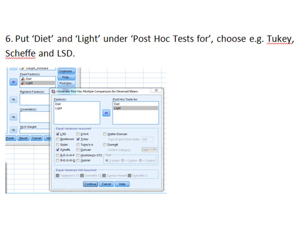
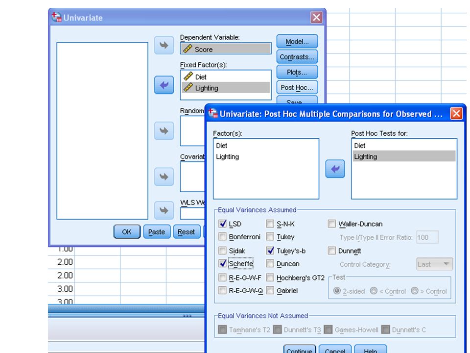
61. Example 1.3.i (aXb factorial, without replication) 5 cages each with 4 rats have been used for a ‘Completely Randomized Two-Factors (a X b factorial) Without Replication Design’ Experiment. The 20 rats had been assigned randomly to be subjects for the ‘combinations’ of factor one (Diet A, B, C, D) with factor 2 (Lighting 1, 2, 3, 4, 5). The response is ‘score’ after the twenty ‘treatments’ e.g. a growth in weight within a certain period of time. Please find any Significant Differences caused by the two factors.

68. Example 1.3.ii (aXb factorial, with replication) - Subjects are randomly chosen into each ‘combination’ of the two factors under investigation, with replications for each combination. The researcher is interested in both factors. - Due to replication, error term and its df are no longer zero, this facilitate calculation of Post Hoc Test for Multiple Comparisons of sign. differences among group means.

69. 6 cages each with 4 rats have been used for a ‘Completely Randomized Two-Factors (a x b factorial) With Replication Design’Experiment. The 24 rats had been assigned randomly to be subjects for the ‘combinations’ of factor one (Diet A, B, C, D) with factor two (Lighting 1, 2, 3). The response is a ‘score’ after the ‘treatments’ e.g. a growth in body weight within a certain period of time. Please find any Significant Differences caused by the two factors. If found, where?

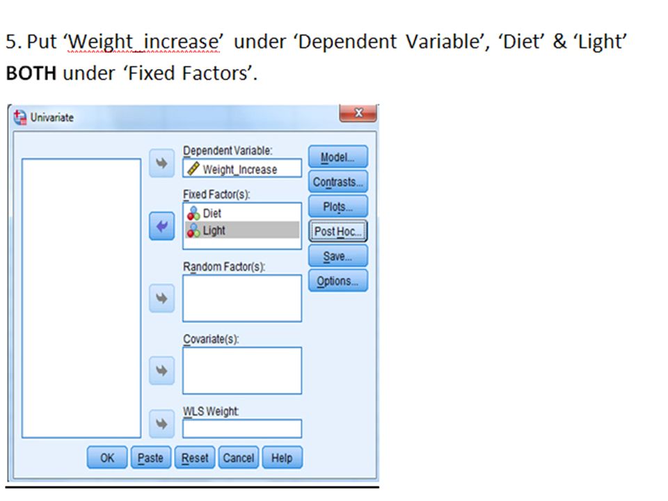
75. Remark – Both factors A and B are ‘FIXED’ factors!

77. Important Supplementary Documents for Interaction For any factorial designs with/without replication, there might be an interaction effect besides the main effects of factors. Document 1 on the attached CD offers a simple method for determining whether there is interaction or not! Please read P. 196 also! For designs without replication, either blocked or factorial, the residual sum of error might contain both interaction effect and random sampling error. Due to no replication, we generally cannot estimate how much error is due to interaction and how much error is due to sampling! So, we had better not to use this design if interaction is suspected among the main factors! However, we might still try to run a test on ‘Simple main effect’ to estimate whether the deviation from perfect case without interaction is purely due to chance or not! Please refer to Document 2 for this!

78. Extreme case is used again! Imagine replication occurs for the previous extreme case:-

79. By intention, the mean of the replication values are equal to the original values without replication! 1.75 2.25 2.75 3.25 3.75 4.25 4.75 5.25 2.85 3.15 3.85 4.15 4.85 5.15 5.85 6.15 3.95 4.05 4.95 5.05 5.95 6.05 6.95 7.05

80. Treatment AB CD Cage 3 Cage 2 Cage 1

83. Same as in extreme case without replication – lines 100% parallel, no interaction, random error exists due to replication but not affecting any Anova results, due to the extreme condition that the average value equal to the original value……. ***This step proves that Sampling Error can now be calculated once there is replication in this factorial design !!

84. Let’s go back to the real case below:-

85. aXb factorial – with replication Treatment (Diet) ABDC Light 3 Light 2 Light 1

86. Comparing the previous graph (below) Treatment AB CD Cage 3 Cage 2 Cage 1

87. Comparing real case with extreme case for aXb factorial with replication There are 3 treatment components and one random error component:- *****COMPUTE ‘3’ = TOTAL ERROR – ‘1’ – ‘2’ – ‘4’***** Where:- 1. Mean differences due to factor a – can be calculated as in extreme case 2. Mean differences due to factor b – can be calculated as in extreme case 3. Mean differences due to effect of combination of factor a and b – No more = ZERO as in extreme case (lines absolutely parallel) 4. Random error component – can be calculated as in extreme case

89. Diet*Light = Corrected Total – Diet – Light – Error = 1043.1-386.5-462.3-125 = 69.3

90. Signification of Interaction between two factors – Lines crossing over =: Significant!! Treatment (Diet) ABCD Light 3 Light 2 Light 1 (average of 27, 35 = 32) (average of 30,40 = 35) (average = 33, 43 = 38) Once crossing occurs, the significance of the interaction would increase rapidly to < 0.05!

92. For average = 32

93. For average = 35

94. For average = 38

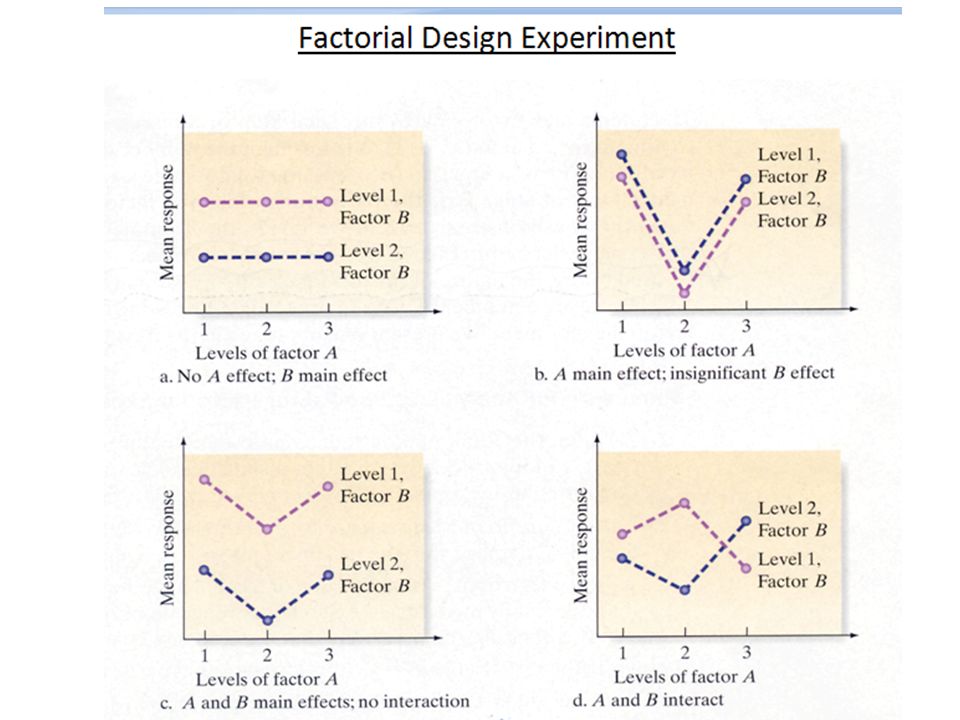
95. Interaction in factorial design The 3 hypothesis Tests The first two hypothesis tests are called tests for the main effects. The null hypothesis is that there are no differences among the levels of the factors. The third hypothesis test is called the test for the interaction, since it examines the effects of the combination of the two factors.

96. Why test for interaction? Interaction being significant is usually a rather disappointing instead of exciting finding, since it would indicate that significant results for the main effect of factors not so easily explained! We might need to do experiments with separate gender due to interaction of gender with treatment being significant, for example! But sometimes it is useful to find interaction, for some purposes with special experimental design e.g. a researcher might want to find an optimum combination of several factors to be the best choice, such as the combined use of vaccines.

98. Fixed and Random Factors A factor would be a fixed factor if exactly the same items must be used again, in case the researcher is required to repeat the experiment e.g. the methods for improving yields or scores, there are only N methods of interest. A factor would be a random one if the research can choose another individual or subjects, in repeating an experiment, e.g. a researcher might just want to know whether different teachers would cause different scores. There is no need to use the same teachers when repeating the experiment. (Whatever inference made from this experiment can be extended to the entire population of all teachers.)

99. The F test equations would be different for fixed and random effects in two-way designs with replication (or in higher level design). If both effects are fixed, their mean squares are compared with the residual mean square. If both effects are random, their mean squares are compared with the interaction rather than the residual mean square. If one effect is random and the other fixed, it is the other way round; the random effect mean square is compared with the residual mean square, and the fixed effect mean square with the interaction. But SPSS still use interaction as denominator for random effect!! **Remark – Therefore, it would be better if the F obtained is greater that the critical F value using both of these two denominators!!

100. For ‘Method’ being fix and ‘Teacher’ being random