1. ECN741: Urban Economics Testing Urban Models

2. ▫Approaches  1. Estimate P{u}  2. Estimate R{u} (land rent)  3. Estimate D {u} (density)  4. Bring in buyer perceptions  5. Estimate theoretically derived envelopes

3. Testing Urban Models ▫Approaches  1. Estimate P{u}  2. Estimate R{u} (land rent)  3. Estimate D {u} (density)  4. Bring in buyer perceptions  5. Estimate derived envelope and bid functions

4. Testing Urban Models ▫Dozens of studies include distance to CBD as an explanatory variable.  Some include actual commuting time (available in the census), which is endogenous! ▫Examples of recent studies that look at several different ways of measuring time or distance:  Ottensmann, John R., Seth Payton, and Joyce Man. 2008. “Urban Location and Housing Prices within a Hedonic Model.” Journal of Regional Analysis and Policy 38 (1):19-35.  Waddell, Paul, Brian J. L. Berry, and Irving Hoch. 1993. “Residential Property Values in a Multinodal Urban Area: New Evidence on the Implicit Price of Location.” The Journal of Real Estate Finance and Economics 7 (2) (September): 117-141.

5. Testing Urban Models ▫These studies do not use theory to derive functional forms. ▫Moreover, many of them forget the most basic fact about an envelope: Moving along the envelope reflects both a change in bids from a given household type and a change from one household type to another: bidding and sorting!  The coefficient of a time or distance variable does not indicate household willingness to pay for access to jobs.  A point on a nonlinear envelope indicates a point on a household’s marginal willingness to pay (i.e. inverse demand function) for access to jobs—a point that depends on the nature of the existing market equilibrium.  But a linear (or semi-log) envelope essentially assumes that no sorting exists and cannot be given a willingness to pay interpretation.

6. Household Heterogeneity Bid Functions Envelope Bid-Rent Functions and Their Envelope

7. Testing Urban Models ▫My early study, which you should ignore, tried to bring in theoretically derived functional forms.  Yinger, John. 1979. “Estimating the Relationship between Location and the Price of Housing.” 1979. Journal of Regional Science, 19 (3) (August): 271 ‑ 286. ▫But the price was too high:  Assumed Cobb-Douglas utility.  Assumed people in a given income-taste class lived in a ring around the CBD.  Ignored non-central worksites.

8. Testing Urban Models ▫Approaches  1. Estimate P{u}  2. Estimate R{u} (land rent)  3. Estimate D {u} (density)  4. Bring in buyer perceptions  5. Estimate derived envelope and bid functions

9. Testing Urban Models ▫Land rent summarizes the derived demand for land, and some studies estimate R{u} instead of P{u}.  Example: D.P. McMillen, 1996. "One Hundred Fifty Years of Land Values in Chicago: A Nonparametric Approach," JUE, (July), pp. 100-124. ▫These studies do not use theoretically derived functional forms.

10. Testing Urban Models ▫Approaches  1. Estimate P{u}  2. Estimate R{u} (land rent)  3. Estimate D{u} (density)  4. Bring in buyer perceptions  5. Estimate derived envelope and bid functions

11. Testing Urban Models ▫A huge literature, going back to the 1950s, estimates population density functions, D{u}. ▫A fairly recent review can be found in:  K.A. Small and S. Song, 1994. "Population and Employment Densities: Structure and Change," JUE, (November), pp. 292-313. ▫There is not much theory in this literature, apart from the (incorrect) derivation of the exponential form from an urban model, which we discussed in an earlier class.

12. Testing Urban Models ▫Some informal theory is offered in the case of multiple worksites. ▫The paper below identifies three assumptions: that different worksites are substitutes, complements, or somewhere in between.  Heikkila, E., P. Gordon, J. I. Kim, R. B. Peiser, H. W. Richardson, and D. Dale-Johnson. 1989. “What Happened to the CBD-Distance Gradient?: Land Values in a Policentric City.” Environment and Planning A 21 (2): 221-232. ▫Allocating each household to a worksite, as in the models discussed earlier, is an example of the first assumption.

13. Testing Urban Models ▫Approaches  1. Estimate P{u}  2. Estimate R{u} (land rent)  3. Estimate D{u} (density)  4. Bring in buyer perceptions  5. Estimate derived envelope and bid functions

14. Testing Urban Models ▫Another way to think about the issue here is that it concerns home buyer perceptions. ▫What information do home buyers have about the time or distance to work sites? ▫Do they care about time or distance? ▫Do they care only about time or distance to one worksite, or do they care about many worksites because the household has multiple workers, might change jobs in the future, or might sell to someone with a different worksite?

15. Testing Urban Models ▫These questions have led me to define as many reasonable time and distance measures as I can with my Cleveland data. ▫And then to determine which ones work the best. ▫In other words, I want the data to answer the above questions. ▫I have identified 9 distance and 9 time measures:

16. Testing Urban Models Table 2. Distance and Time Measures Distance Definition (Miles)MeanMinimumMaximum Distance 1Straight-line distance to Terminal Tower 13.391.1141.36 Distance 2Straight-line distance to downtown worksite 13.570.7342.25 Distance 3Straight-line distance to assigned worksite 6.920.0142.25 Distance 4Average actual straight-line commuting distance 7.973.0129.04 Distance 5Employment-weighted straight-line distance to 5 major worksites13.207.2739.52 Distance 6Distance to Terminal Tower along streets 15.511.4054.60 Distance 7Distance to downtown worksite along streets 15.271.2055.40 Distance 8Distance to assigned worksite along streets 8.680.0055.40 Distance 9Employment-weighted distance to 5 major worksites along streets10.832.7545.66 Time Definition (Minutes)MeanMinimumMaximum Time 1Estimated time to Terminal Tower 44.519.8787.48 Time 2Estimated time to downtown worksite 45.4733.8960.90 Time 3Estimated time to assigned worksite 32.334.24121.39 Time 4Average actual commuting time 25.8711.1146.53 Time 5Employment-weighted estimated time to 5 major worksites46.3125.9786.26 Time 6Time to Terminal Tower along streets 25.515.0062.00 Time 7Time to downtown worksite along streets 25.025.0060.00 Time 8Time to assigned worksite along streets 17.372.0085.00 Time 9Employment-weighted time to 5 major worksites along streets25.9713.3456.21 Speed Definition (MPH)MeanMinimumMaximum Speed 1Implied average speed to Terminal Tower16.146.1028.37 Speed 2Implied average speed to downtown worksite17.041.2941.62 Speed 3Implied average speed to assigned worksite10.550.0641.62 Speed 4Implied average actual commuting speed18.687.5976.28 Speed 5Implied employment-weighted estimated speed to 5 major worksites16.309.0428.81 Speed 6Implied average speed to Terminal Tower on streets34.342.8658.89 Speed 7Implied average time to downtown worksite on streets34.673.1659.27 Speed 8Implied average speed to assigned worksite on streets22.370.0358.46 Speed 9Implied employment-weighted speed to 5 major worksites on streets22.725.1751.18

17. Testing Urban Models ▫One tricky issue is how to allocate households to worksites for Distance 3 and Time 3.  Recall that finding the boundaries between the residential zones of suburban and central city workers is pretty complicated.  But the allocation problem in this case is not so complicated because we already know (1) how many workers are at each worksite and (2) how many households live in each neighborhood (CBG).  So the idea is just to pick the closest CBGs until there are enough people to fill the jobs at each worksite.

18. Testing Urban Models Miles from CBD

20. Testing Urban Models ▫Which Measure Is Best?  Time has the advantage over distance that it accounts for actual routes, mode choice, and congestion.  Distance has the advantage over time that it incorporates operating costs.  Distance also may be more easily perceived by a house buyer. But we really do not know what people perceive—that is, what information about commuting costs they rely on when they make a housing bid. Maybe everyone uses Google maps!

21. Testing Urban Models ▫Approaches  1. Estimate P{u}  2. Estimate R{u} (land rent)  3. Estimate D{u} (density)  4. Bring in buyer perceptions  5. Estimate derived envelope and bid functions

22. Testing Urban Models ▫Controls  These results given below come from a regression with many controls for housing characteristics, neighborhood characteristics, and public services.  More on this later!  The initial regression has about 23,000 house sales and 1,665 neighborhood (CBG) fixed effects.  The housing price (= P{u} ) regression is based on 1,665 neighborhoods (CBGs).

23. Testing Urban Models Table 3. Correlations for Distance and Time Measures Dist 1Dist 2Dist 3Dist 4Dist 5Dist 6Dist 7Dist 8Dist 9 Distance 11.00 Distance 20.991.00 Distance 30.710.731.00 Distance 40.640.630.551.00 Distance 50.970.980.790.621.00 Distance 60.790.800.660.560.781.00 Distance 70.770.790.660.530.780.961.00 Distance 80.640.650.870.580.690.720.731.00 Distance 90.790.800.790.600.820.910.920.851.00 Time 1Time 2Time 3Time 4Time 5Time 6Time 7Time 8Time 9 Time 11.00 Time 20.701.00 Time 30.300.571.00 Time 4-0.030.070.281.00 Time 50.820.870.610.101.00 Time 60.950.670.340.060.781.00 Time 70.940.680.340.040.760.991.00 Time 80.610.540.660.250.660.700.711.00 Time 90.900.790.520.100.890.940.950.761.00

24. Testing Urban Models Semi-Log Bid-Price Function Envelopes, Part 1 Distance MeasureCoefficientt-StatisticR-Squared Distance 1-0.0070482-4.580.7142 Distance 2-0.0069594-4.610.7143 Distance 3-0.0061207-4.390.7138 Distance 4-0.0018316-0.820.7103 Distance 5-0.0078257-4.810.7145 Distance 6-0.0015973-1.840.7110 Distance 7-0.0012967-1.550.7108 Distance 8-0.0023002-2.430.7118 Distance 9-0.0019577-2.010.7112

25. Testing Urban Models Semi-Log Bid-Price Function Envelopes, Part 2 Time MeasureCoefficientt-StatisticR-Squared Time 1-0.0043931-4.460.7145 Time 2-0.0030373-1.720.7112 Time 3-0.0008516-1.890.711 Time 4-0.0027473-2.210.7113 Time 5-0.0040401-4.590.7145 Time 6-0.0029835-2.310.7115 Time 7-0.0023512-1.820.711 Time 8-0.0022187-2.190.7115 Time 9-0.0041787-2.940.7121

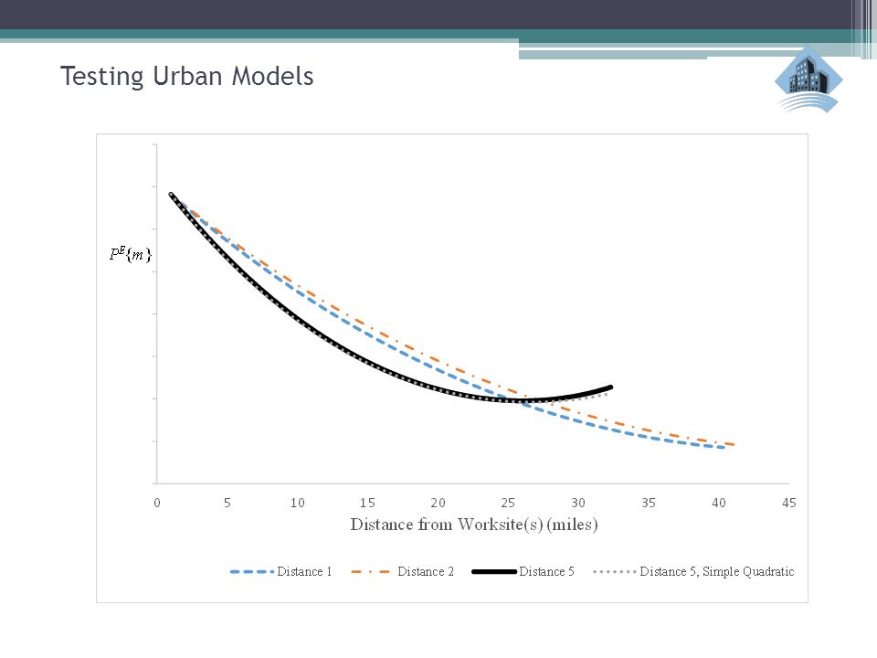
26. Testing Urban Models ▫The next step is to estimate theoretically derived bid-price function envelopes. ▫These are the envelopes covered in the slides and notes on household heterogeneity. ▫The regressions on which these pictures are based work very well, with highly significant coefficients for the two variables that define the envelope, which were derived in an earlier class—but they are preliminary! ▫Distance 5 works best and distance works better than time, but the differences in SSE are small.

27. Testing Urban Models

30. ▫A Big Puzzle: Many of these envelopes turn up for the longest commutes.  I do not know what this means.  It could mean that some people actually enjoy commuting.  It could mean that I have an omitted variable that is highly correlated with distance, such as peace and quiet.  Note that this puzzle show up in the simple quadratic forms, too—it is not a product of my functional form.

31. Testing Urban Models ▫The next step: Look for normal sorting.  The functional form used in these estimations makes it possible to separate bidding and sorting.  It also makes it possible to test for normal sorting: that is, do higher-income households tend to live in more distant locations. This test was described in an earlier class.  I have not conducted these tests yet, but will let you know if I get to them this fall.