1. Transient Conduction: Finite-Difference Equations and Solutions Chapter 5 Section 5.9  

2. Finite-Difference Method The Finite-Difference Method An approximate method for determining temperatures at discrete (nodal) points of the physical system and at discrete times during the transient process. Procedure: ─ Represent the physical system by a nodal network, with an m, n notation used to designate the location of discrete points in the network, ─ Use the energy balance method to obtain a finite-difference equation for each node of unknown temperature. ─ Solve the resulting set of equations for the nodal temperatures at t = ∆t, 2∆t, 3∆t, …, until steady-state is reached. What is represented by the temperature, ? and discretize the problem in time by designating a time increment ∆t and expressing the time as t = p∆t, where p assumes integer values, (p = 0, 1, 2,…).

3. Storage Term Energy Balance and Finite-Difference Approximation for the Storage Term For any nodal region, the energy balance is (5.76) where, according to convention, all heat flow is assumed to be into the region. Discretization of temperature variation with time: Finite-difference form of the storage term: Existence of two options for the time at which all other terms in the energy balance are evaluated: p or p+1. (5.69)

4. Explicit Method The Explicit Method of Solution All other terms in the energy balance are evaluated at the preceding time corresponding to p. Equation (5.69) is then termed a forward-difference approximation. Example: Two-dimensional conduction for an interior node with ∆x=∆y. (5.71) Unknown nodal temperatures at the new time, t = (p+1)∆t, are determined exclusively by known nodal temperatures at the preceding time, t = p∆t, hence the term explicit solution.

5. Explicit Method (cont.) How is solution accuracy affected by the choice of ∆x and ∆t? Do other factors influence the choice of ∆t? What is the nature of an unstable solution? Stability criterion: Determined by requiring the coefficient for the node of interest at the previous time to be greater than or equal to zero. Hence, for the two-dimensional interior node: Table 5.2 finite-difference equations for other common nodal regions. For a finite-difference equation of the form,

6. Implicit Method The Implicit Method of Solution All other terms in the energy balance are evaluated at the new time corresponding to p+1. Equation (5.69) is then termed a backward-difference approximation. Example: Two-dimensional conduction for an interior node with ∆x=∆y. (5.87) System of N finite-difference equations for N unknown nodal temperatures may be solved by matrix inversion or Gauss-Seidel iteration. Solution is unconditionally stable. Table 5.2 finite-difference equations for other common nodal regions.

7. Marching Solution Transient temperature distribution is determined by a marching solution, beginning with known initial conditions. 1 ∆t------ …………… -- Known 22∆t------ …………… -- 3 3∆t------ …………… --...... Steady-state -------- ……………. -- ptT 1 T 2 T 3……………….. T N 00T 1,i T 2,i T 3,i………………. T N,i

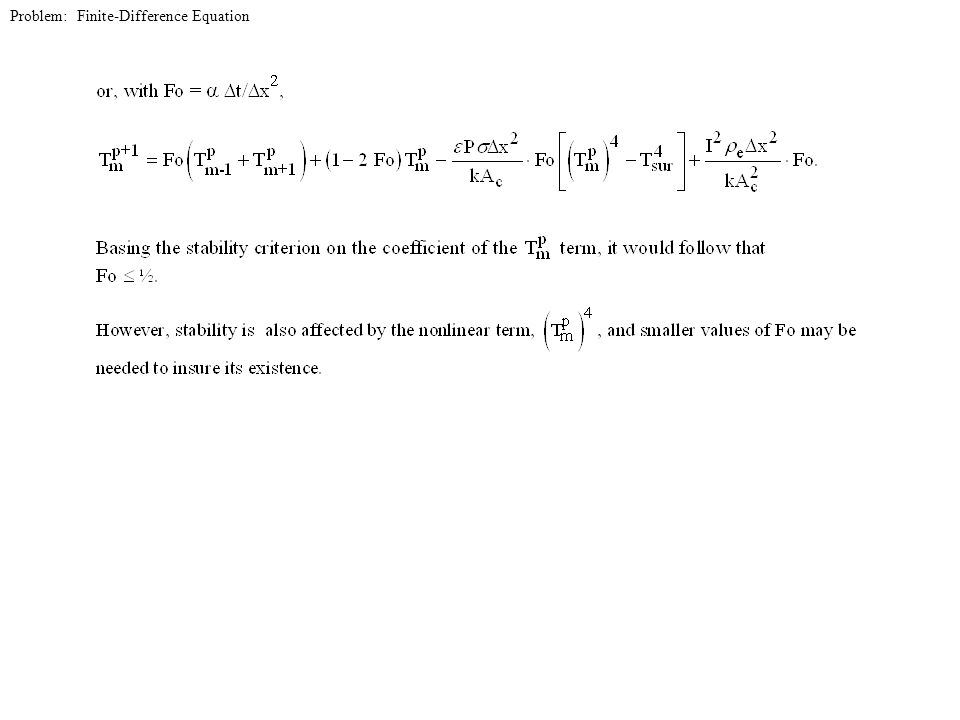
8. Problem: Finite-Difference Equation Problem 5.94: Derivation of explicit form of finite-difference equation for a nodal point in a thin, electrically conducting rod confined by a vacuum enclosure.

9. Problem: Finite-Difference Equation

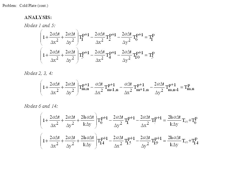
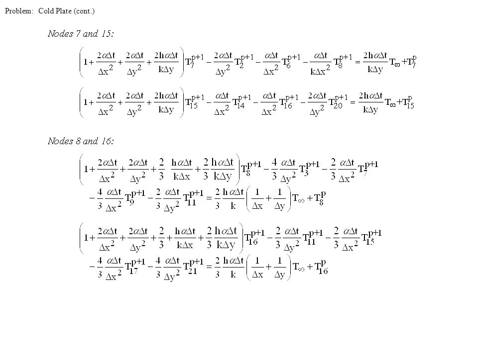
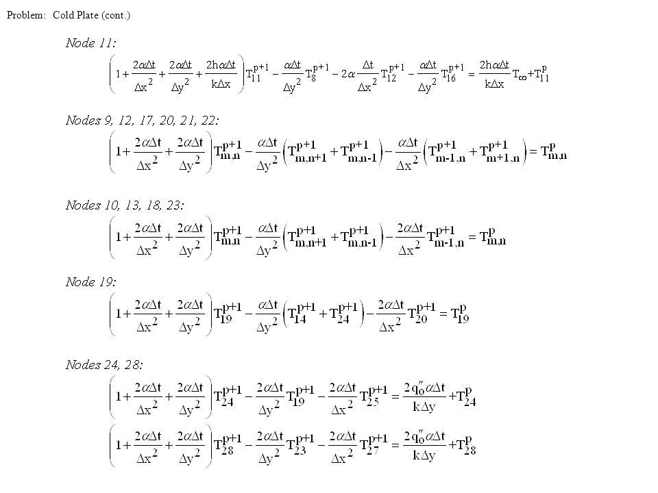
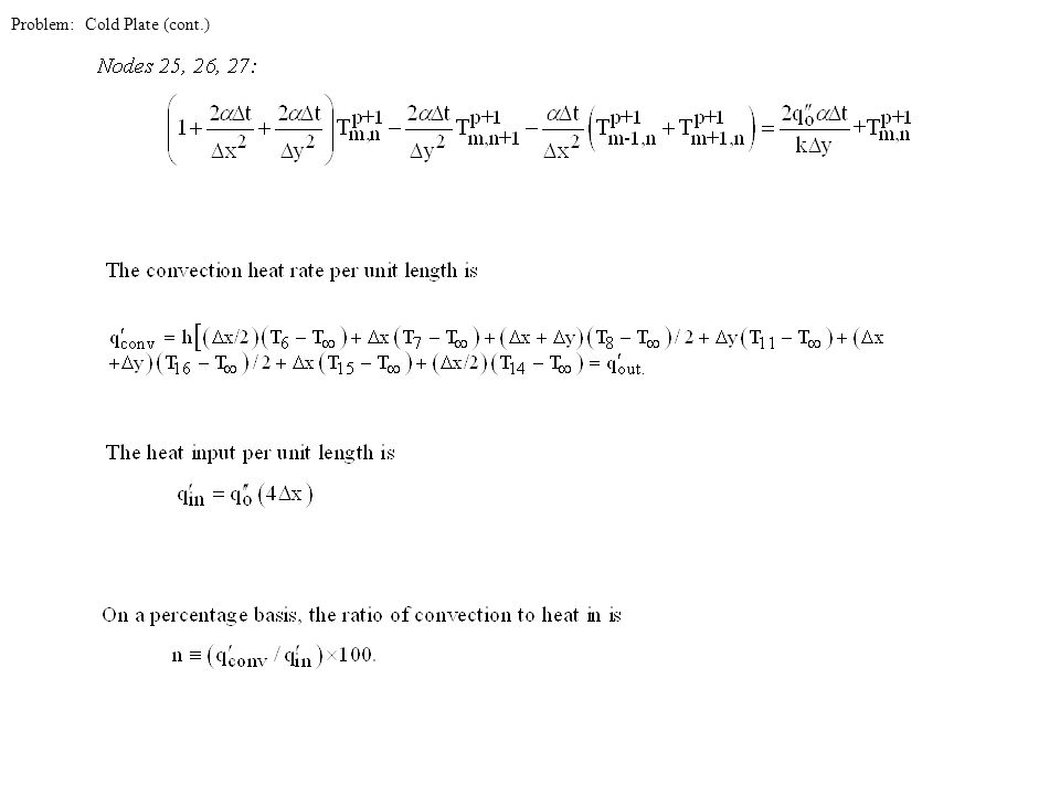
11. Problem: Cold Plate Problem 5.127: Use of implicit finite-difference method with a time interval of ∆t = 0.1s to determine transient response of a water-cooled cold plate attached to IBM multi-chip thermal conduction module. Features: Cold plate is at a uniform temperature, T i =15°C, when a uniform heat flux of is applied to its base due to activation of chips. During the transient process, heat transfer into the cold plate increases its thermal energy while providing for heat transfer by convection to the water. Steady state is reached when.

12. Problem: Cold Plate (cont.)