1. Interannual Variability in the ChEAS Mesonet ChEAS XI, 12 August 2008 UNDERC-East, Land O Lakes, WI Ankur Desai Atmospheric & Oceanic Sciences, University of Wisconsin-Madison

2. What’s the Deal? Interannual variation (IAV) in carbon fluxes from land to atmosphere are significant at most flux sites Key to understanding how climate affects ecosystems comes from modeling IAV IAV (years-decade) is currently poorly modeled, while hourly, seasonal, and even successional (century) are better

3. Can we simulate this?

4. Sipnet A “simplified” model of ecosystem carbon / water and land-atmosphere interaction –Minimal number of parameters –Driven by meteorological forcing Still has >60 parameters Braswell et al., 2005, GCB Sacks et al., 2006, GCB added snow Zobitz et al., 2008

5. Results

6. 2 years = 7 years 199719981999200020012002200320042005

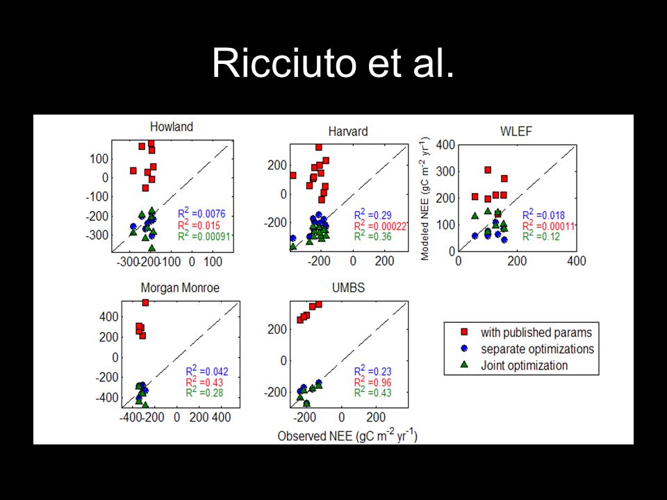
7. Ricciuto et al.

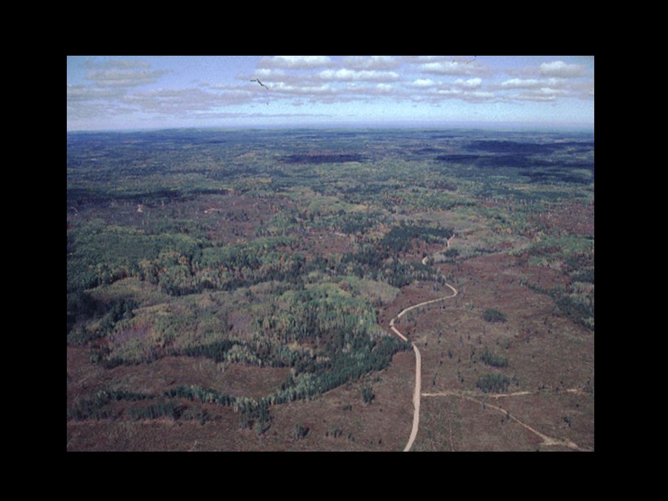
9. Our region

10. Any coherence? Desai et al, 2008, Ag For Met

11. Cross-site IAV Hypothesis: IAV in flux towers in the same region are coherent in time Hypothesis: Simple climate driven models can explain this IAV –Growing season length –Climate thresholds –Mean annual precip

12. A whole bunch of data

13. Coherence?

14. Growing season and IAV Does growing season start explain IAV? Can a very simple model be constructed to explain IAV? –Hypothesis: growing season length explains IAV Can we make a cost function more attuned to IAV? –Hypothesis: MCMC overfits to hourly data

15. Hello again

16. The model Driven by PAR, Air and Soil T, VPD, (Precip) LUE based GPP model f(PAR,T,VPD) Three respiration pools f(T, GPP) Output: NEE, ER, GPP, LAI Sigmoidal GDD function for leaf out Sigmoidal Soil T function for leaf off 17 parameters, 3 are fixed Desai et al., in prep (a)

17. The optimizer All flux towers with multiple years of data Estimate parameters with Markov Chain Monte Carlo (smart random walk) Written in IDL

18. MCMC MCMC is an optimizing method to minimize model-data mismatch –Quasi-random walk through parameter space (Metropolis) Start at many random places (Chains) in prior parameter space –Move “downhill” to minima in model-data RMS by randomly changing a parameter from current value to a nearby value –Avoid local minima by occasionally performing “uphill” moves in proportion to maximum likelihood of accepted point –Use simulated annealing to tune parameter space exploration –Pick best chain and continue space exploration –Requires 100,000-500,000 model iterations (chain exploration, spin-up, sampling) –End result – “best” parameter set and confidence intervals (from all the iterations) –Cost function compared to observed NEE

19. New cost function Original log likelihood computes sum of squared difference at hourly timestep What if we also added monthly and annual squared differences to this likelihood? Have to scale these less frequent values Have to deal with missing data

20. I like likelihood

26. Regional IAV How well do we know regional (scaled-up) IAV? Do top-down and bottom-up regional flux estimation techniques agree on IAV (if not magnitude)? What controls regional IAV? –Wetland IAV vs Upland IAV Step 1: Scale the towers

28. Heterogeneous footprint

29. Scaling with towers NEP (=-NEE) at 13 sites Stand age matters Ecosystem type matters Is interannual variability coherent? Are we sampling sufficient land cover types”?

30. Desai et al., 2008, AFM Multi-tower synthesis aggregation –parameter optimization with minimal 2 equation model

31. Tall tower downscaling Wang et al., 2006

32. Scaling evaluation Desai et al., 2008

33. Next step Use our IAV model with all 17 (19) flux towers - estimate parameters for each Use better landcover and better age distribution from NASA project Upscale again - this time over long time period This experiment for Northern Highlands 1989-2007 (Buffam et al., in prep)

36. Many years of flux

37. Regional coherence? Desai et al., in prep

38. Regional coherence?

39. Conclusions There is some coherence in IAV across ChEAS –Better statistical method to show this? A simple model with explicit phenology can capture the IAV across sites only with a better likelihood function –Next step: Simple model with fixed phenology Limited convergence on IAV from regional methods

40. Other things Sulman et al., in prep - the role of wetlands in regional carbon balance Lake Superior carbon balance from ABL budgets (Atilla, McKinley) - Urban et al, in prep Small lakes in the landscape (Buffam, Kratz) Successional trends and modeling (Dietze) Hyperspectral remote sensing (Townsend, Serbin, Cook) Top-down CO2 budgets in valeys and complex terrain (Stephens, Schimel, Bowling, deWekker) CH4 (pending), advection (pending - Yi), urban micromet and biogeochem (pending) NEON? (Schimel, UNDERC)

41. Thanks Desai lab: http://flux.aos.wisc.eduhttp://flux.aos.wisc.edu –Ben Sulman, Jonathan Thom, Shelly Knuth DOE NICCR, NSF, UW, DOE, NASA, USFS, Northern Research Station, Kemp NRS All the tower people