1. Chapter 13, Sterman: Modeling Decision Making Powerpoints by: James Burns

2. Modeling Decision Making This chapter explores the formulation of the decision rules representing the behavior of the agents.

3. Principles All model structures consist of two parts: –Assumptions about the physical and institutional environment –Assumptions about the decision processes of the agents

5. The physical/institutional structure… Includes the model boundary and stock and flow structures of people, material, money, information, and so forth that characterize the system Forrester’s Urban Dynamics sought to understand why America’s large cities continued to decay despite massive amounts of aid and numerous renewal programs

6. The decision processes of the agents… Refer to the decision rules that determine the behavior of the actors in the system In Urban Dynamics, these included decision rules governing migration and construction

7. Actually portraying the physical and … Institutional structure of a system is relatively straightforward.

8. Representing the decision rules of actors is … Subtle and challenging To be useful simulation models must mimic the behavior of the real decision makers so that they respond appropriately, not only for conditions observed in the past but also for circumstances never yet encountered

9. Decisions and Decision Rules Modelers must make a sharp distinction between decisions and decision rules Decision rules are the policies and protocols specifying how the decision maker processes available information Decisions are the outcome of this process

10. More Decisions and Decision Rules It is not sufficient to model a particular decision. Modelers must detect and represent the guiding policy that yields the stream of decisions Every rate in the stock and flow structure constitutes a decision point, and –The modeler must specify precisely the decision rule determining the rate

11. Every Decision Rule… Can be thought of as an information processing procedure The inputs to the decision process are various types of information or cues –The cues are then interpreted by the decision maker to yield the decision –Decision rules may not use all available information

12. Cues in the Department Store Case Cues used to revise prices in the department store case include wholesale costs, inventory turnover, and competitor prices Department store pricing decisions do not depend on interest rates, required rates of return, store overhead, trade-offs of holding costs against the risk of stock- outs, estimates of the elasticity of demand, or any sophisticated strategic reasoning.

13. This gets back to a strategic modeling question… Is our model a descriptive model or is it a prescriptive one? Recall: –Descriptive models…tell it like it actually is –Prescriptive models…tell is like it should be

14. What determines what information gets used? Mental models of the decision makers Organizational, political, personal, and other factors, influence the selection of cues from the set of available information The cues (information) used is not necessarily processed optimally

15. According to Nobel Laureate Gary Becker… All human behavior can be viewed as involving participants who maximize their utility from a stable set of preferences and accumulate an optimal amount of information

16. In Becker’s view… Not only do people make optimal decisions given the information they have, but they also invest exactly the optimal time and effort in the decision process, ceasing their deliberations when the expected gain to further effort equals the cost

17. Five Formulation Fundamentals The Baker Criterion: The inputs to all decision rules in models must be restricted to information actually available to the real decision makers Senator Howard Baker: What did he (Nixon) know and when did he know it??

18. In modeling decision rules… Must ask, “What did they know and when did they know it?” To properly mimic the behavior of a real system, a model can use as an input to a decision only those sources of information actually available to and used by the decision makers in the real system

19. The principle that decisions in models must be based on available information has three corollaries First, no one knows with certainty what the future will bring Second, perceived and actual conditions often differ Third, modelers cannot assume decision makers know with certainty the outcomes of contingencies they have never experienced

20. The decision rules of a model should conform to managerial practice All variables and relationships should have real world counterparts and meaning The units of measure in all equations must balance without the use of arbitrary scaling factors Decision making should not be assumed to conform to any prior theory but should be investigated firsthand

21. Homework: Examine and respond to the Challenge questions on pages 520 to 522

22. A Library of Common Formulations Of rate equations Are presented next Are the building blocks from which more realistic and complex structures can be derived

23. Formulating Rate Equations Fractional Increase Rate Fractional Decrease Rate Adjustment to a goal

24. Fractional Increase Rate R I = g * S Here, R I is an input rate, g is some fraction (<1) and S is the stock that accumulates R I Examples Birth rate = birth rate normal * Population Interest Due = Interest Rate * Debt Outstanding

25. Fractional Increase Rate These examples all generate first- order, ________ loops. By themselves, these rates create exponential growth It’s never a good practice for these rates to be anything other than non- negative

26. Fractional Decrease Rate R O = g * S R O = g * S Here, R O is an output rate, g is some fraction (<1) and S is the stock that is depleted by R O Examples Death rate = death rate normal * Population Death rate = Population / Average Lifetime

27. Fractional Decrease Rate Left to themselves these rates generate exponential decay Left to themselves, these rates create first-order, negative feedback loops

28. Adjustment to a goal R I = Discrepancy / AT = (S* - S) / AT Examples –Change in Price = (Competitors price – Price) / Price Adjustment time –Net Hiring Rate = (Desired Labor – Labor) / Hiring Delay –Bldg heat loss = (outside temp – inside temp) / temp adjustment time

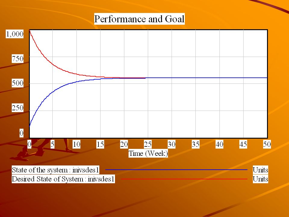
29. Adjustment to a Goal Generates exponential goal-seeking behavior Is also considered a first-order, negative feedback loop Often the actual state of the system is not known to decision makers who rely instead on perceptions or beliefs about the state of the system –In these cases, the gap is the difference between the desired and the perceived state of the system

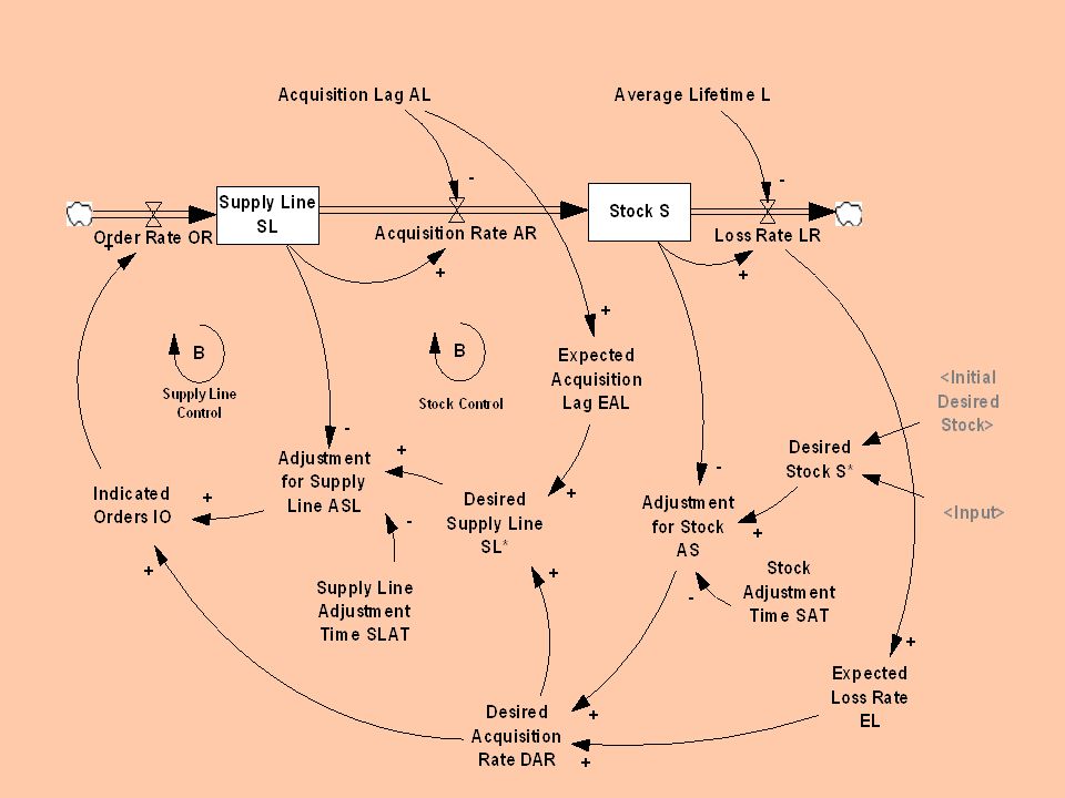
30. More Formulating Rate Equations The Stock Management Structure: Rate=Normal Rate + adjustments Flow = Resource * Productivity Y = Y * Effect of X1 on Y * Effect of X2 on Y* … * Effect of Xn on Y

31. Stock Management Structure Rate = Normal Rate + Adjustments If the input rate is R I = (S* - S) / AT, and the output rate is R O, then the steady state equilibrium will be S = S* - R O * AT To prevent this the stock management structure adds the expected outflow to the stock adjustment to prevent the steady state error: Inflow = Expected outflow + Adjustment for Stock

32. Flow = Resource * Productivity The flows affecting a stock frequently depend on resources other than the stock itself The rate is determined by a resource and the productivity of that resource Rate = Resource * Productivity, or Rate = Resource/Resources Required per Unit Produced

33. Examples Production = Labor Force * Average Productivity

34. Y = Y * Effect of X1 on Y * Effect of X2 on Y* … * Effect of Xn on Y These are called MULTIPLICATIVE EFFECTS Examples: Rate = Normal Fractional Rate * Stock * Effect of X1 on Rate * … * Effect of Xn on Rate Birth Rate = Birth Rate Normal * Population * Effect of Material on Birth Rate * Effect of Pollution on Birth Rate * Effect of Crowding on Birth Rate * Effect of Food on Birth Rate

35. Recall, Forrester’s world2 Model… A reference year of 1970 was defined Normal fractional birth rate was the world average in the reference year All of the effects were normalized to their 1970 values, making those normalized values equal to 1

36. Multiplicative effects Create nonlinearities Forrester really believes the effects are multiplicative As an alternative consider additive effects:

37. Y = Y* + Effect of X1 on Y + Effect of X2 on Y + … + Effect of Xn on Y Example: Change in wage = Fractional Change in Wage * Wage Fractional Change in Wage = Change in Wage from Labor Availability + Change in Wage from Inflation + change in Wage from Productivity + Change in Wage from Profitability + Change in Wage from Equity

38. Multiplicative or Additive, WHICH??? Linear formulations are common because such formulations are simple Multiplicative formulations are generally preferable and sometimes required The actual relationship between births and food, crowding, or pollution is typically complex and nonlinear

39. Multiplicative or Additive, WHICH??? Both are approximations to the underlying, true nonlinear function: Y = f(X1, X2, …, Xn) Each approximation is centered on a particular operating point given by the reference point Y* = f(X1*, X2*, …, Xn*)

40. Both additive and multiplicative approximations… Will be reasonable in the neighborhood of the operating point but increasingly diverge from the true, underlying function as the system moves away from it

41. Additive vs. Multiplicative Additive assumes the effects of each input are strongly separable Strong separability is clearly incorrect in extreme conditions In the birth rate example, births must be zero when food per capita is zero no matter how favorable the other conditions are The additive formulation can never capture this

42. More Formulating Rate Equations Fuzzy MIN Function Fuzzy MAX Function Floating goals

43. Fuzzy MIN Function A rate or auxiliary is determined by the most scarce of several resources Production = MIN(Desired Production, Capacity) Generally, Y = MIN(X, Y*), where Y* is the capacity of the process

44. Problems with the MIN Function The sharp discontinuity created by the MIN function is often unrealistic Often the capacity constraint is approached gradually due to physical characteristics of the system A fuzzy MIN function will accomplish this for us so that there is not sharp discontinuity

45. Fuzzy MAX Function Analogous to fuzzy MIN function Hiring Rate = MAX(0, Desired Hiring Rate) prevents Hiring Rate from ever gong negative Useful in situations where decision makers want to keep a variable Y at its desired rate even as X falls to zero

46. Fuzzy MIN and MAX Functions I couldn’t find any in VENSIM Therefore, you must set this up using a TABLE function

47. Floating goals The goal moves toward the actual state of the system while the actual state of the system moves toward the goal.

48. Floating Goal

50. More Formulating Rate Equations Nonlinear Weighted Average Modeling Search: Hill-Climbing Optimization Resource Allocation

51. Nonlinear Weighted Average

52. Modeling Search: Hill-Climbing Optimization Decision makers must optimize a system but lack knowledge of the system structure that might help them identify the optimal operating point Examples: A firm wants to –maximize profit –Minimize costs –Maximize the mix of labor and capital Can do this in simulated real time using a variant of floating goals

53. To find the optimal mix of labor and capital… The model adjusts the mix in the right direction, toward a desired state. This is called hill-climbing

54. Hill Climbing

55. Modeling Search: Hill-Climbing Optimization I have taught entire courses in hill- climbing optimization My favorite—Powell’s method—also the one used in Vensim –Doesn’t require first-partial derivatives of the objective function, as many methods do –Is fast, giving quadratic convergence –Uses conjugate directions of search

56. Problems with Hill-climbing Optimization Methods Converges to local optima Must start it from a number of different points in the search space to ensure that a global optimum is found But that is NOT WHAT IS GOING ON HERE—THE SIMPLE TECHNIQUE USED HERE IS JUST A VARIANT OF THE 1 ST ORDER NEGATIVE FEEDBACK GOAL SEEKING STRUCTURE

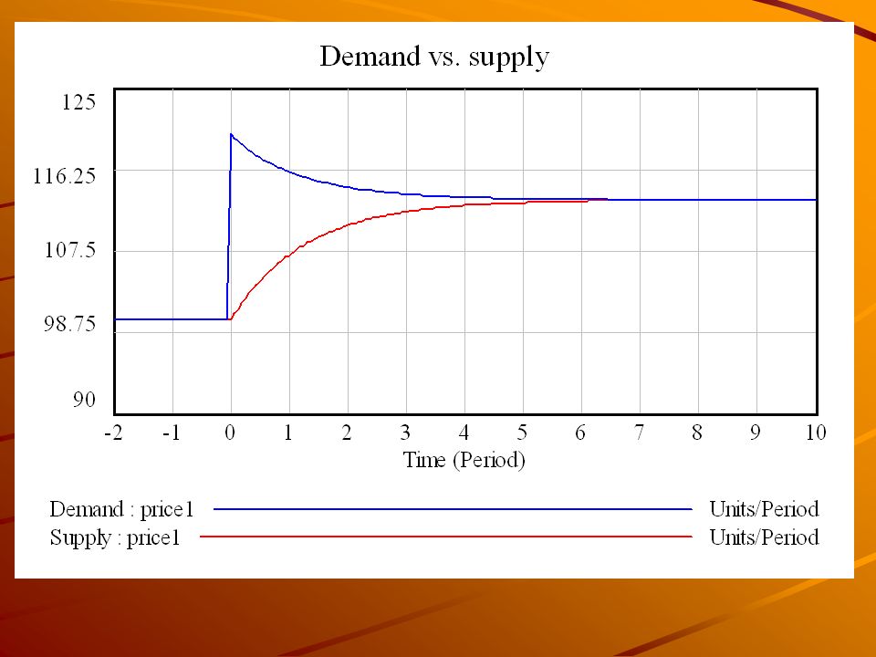
57. Example—setting price

58. Price Decisions

59. Price Adjustment in Hill Climbing Fashion

62. Resource Allocation

64. Common Pitfalls All outflows require First-Order Control Avoid IF..THEN..ELSE Formulations Disaggregate Net Flows

65. All outflows require First-Order Control Real stocks such as inventories, personnel, cash and other resources cannot become negative Outflow rates must be formulated so these stocks remain nonnegative even under extreme conditions Do so requires all outflows to have first-order control

66. First-Order Control Means the outflows are governed by a first-order negative feedback loop that shuts down the flow as the stock drops to zero Examples: –Outflow = MIN (Desired Outflow, Maximum Outflow) –Outflow = Stock / Residence time –Maximum Outflow = Stock / Minimum Residence time

67. Avoid IF..THEN..ELSE Formulations Sterman doesn’t like these because they introduce sharp discontinuities into your models, discontinuities that are often inappropriate. Individual decisions are rarely either/or In many cases the decision is a compromise or weighted average of competing pressures

68. More on IF..THEN..ELSE Formulations They create conditional statements that are often difficult to understand, especially when the conditions are complex or nested with others

69. Disaggregate Net Flows

70. Summary