Download presentation
Presentation is loading. Please wait.

1
Bayesian Decision Theory (Classification) 主講人:虞台文
 主講人:虞台文")
2
Contents Introduction Generalize Bayesian Decision Rule Discriminant Functions The Normal Distribution Discriminant Functions for the Normal Populations. Minimax Criterion Neyman-Pearson Criterion

3
Bayesian Decision Theory (Classification) Introduction
 Introduction")
4
What is Bayesian Decision Theory? Mathematical foundation for decision making. Using probabilistic approach to help making decision (e.g., classification) so as to minimize the risk (cost).
 so as to minimize the risk (cost)..")
5
Preliminaries and Notations a state of nature prior probability feature vector class-conditional density posterior probability

6
Bayesian Rule

7
Decision unimportant in making decision unimportant in making decision

8
Decision Decide i if P( i |x) > P( j |x) j i Decide i if p(x| i )P( i ) > p(x| j )P( j ) j i Special cases: 1. P( 1 )=P( 2 )= =P( c ) 2. p(x| 1 )=p(x| 2 ) = = p(x| c )
=P( 2 )= =P( c ) 2. p(x| 1 )=p(x| 2 ) = = p(x| c ).")
9
Two Categories Decide i if P( i |x) > P( j |x) j i Decide i if p(x| i )P( i ) > p(x| j )P( j ) j i Decide 1 if P( 1 |x) > P( 2 |x); otherwise decide 2 Decide 1 if p(x| 1 )P( 1 ) > p(x| 2 )P( 2 ); otherwise decide 2 Special cases: 1. P( 1 )=P( 2 ) Decide 1 if p(x| 1 ) > p(x| 2 ); otherwise decide 1 2. p(x| 1 )=p(x| 2 ) Decide 1 if P( 1 ) > P( 2 ); otherwise decide 2
=P( 2 ) Decide 1 if p(x| 1 ) > p(x| 2 ); otherwise decide 1 2. p(x| 1 )=p(x| 2 ) Decide 1 if P( 1 ) > P( 2 ); otherwise decide 2.")
10
Example R2R2 P( 1 )=P( 2 ) R1R1
=P( 2 ) R1R1")
11
Example R1R1 R1R1 R2R2 R2R2 P( 1 )=2/3 P( 2 )=1/3 Decide 1 if p(x| 1 )P( 1 ) > p(x| 2 )P( 2 ); otherwise decide 2
=2/3 P( 2 )=1/3 Decide 1 if p(x| 1 )P( 1 ) > p(x| 2 )P( 2 ); otherwise decide 2")
12
Classification Error Consider two categories: Decide 1 if P( 1 |x) > P( 2 |x); otherwise decide 2
 > P( 2 |x); otherwise decide 2")
13
Classification Error Consider two categories: Decide 1 if P( 1 |x) > P( 2 |x); otherwise decide 2
 > P( 2 |x); otherwise decide 2")
14
Bayesian Decision Theory (Classification) Generalized Bayesian Decision Rule
 Generalized Bayesian Decision Rule")
15
The Generation a set of c states of nature a set of a possible actions The loss incurred for taking action i when the true state of nature is j. We want to minimize the expected loss in making decision. Risk can be zero.

16
Conditional Risk Given x, the expected loss (risk) associated with taking action i. Given x, the expected loss (risk) associated with taking action i.
 associated with taking action i..")
17
0/1 Loss Function

18
Decision Bayesian Decision Rule:

19
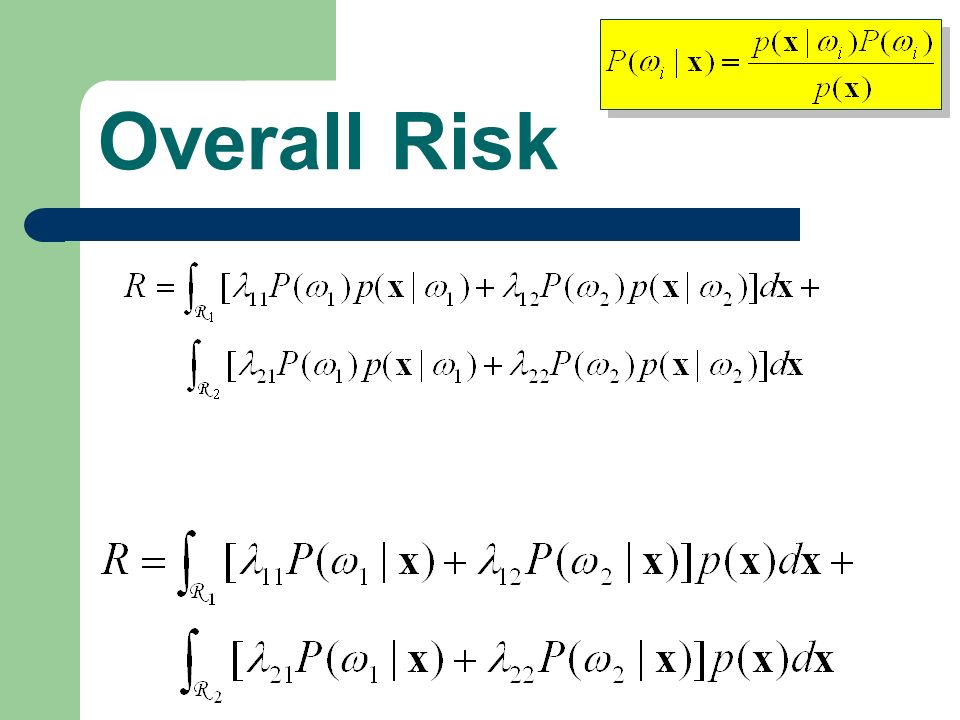
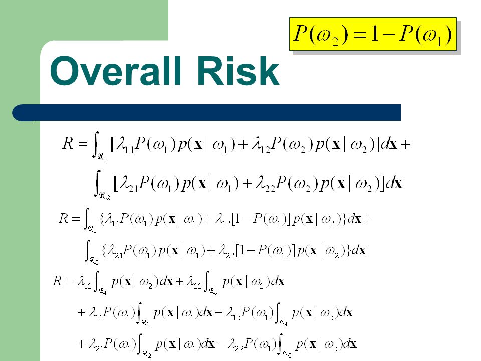
Overall Risk Decision function Bayesian decision rule: the optimal one to minimize the overall risk Its resulting overall risk is called the Bayesian risk

20
Two-Category Classification Action State of Nature Loss Function

21
Two-Category Classification Perform 1 if R( 2 |x) > R( 1 |x); otherwise perform 2
 > R( 1 |x); otherwise perform 2")
22
Two-Category Classification Perform 1 if R( 2 |x) > R( 1 |x); otherwise perform 2 positive Posterior probabilities are scaled before comparison.
 > R( 1 |x); otherwise perform 2 positive Posterior probabilities are scaled before comparison.")
23
Two-Category Classification irrelevan t Perform 1 if R( 2 |x) > R( 1 |x); otherwise perform 2
 > R( 1 |x); otherwise perform 2")
24
Two-Category Classification Perform 1 if Likelihood Ratio Threshold This slide will be recalled later.

25
Bayesian Decision Theory (Classification) Discriminant Functions
 Discriminant Functions")
26
The Multicategory Classification g1(x)g1(x) g1(x)g1(x) g2(x)g2(x) g2(x)g2(x) gc(x)gc(x) gc(x)gc(x) x Action (e.g., classification) (x)(x) Assign x to i if g i (x) > g j (x) for all j i. g i (x)’s are called the discriminant functions. How to define discriminant functions?
’s are called the discriminant functions. How to define discriminant functions .")
27
Simple Discriminant Functions Minimum Risk case: Minimum Error-Rate case: If f( . ) is a monotonically increasing function, than f(g i ( . ) )’s are also be discriminant functions.
 is a monotonically increasing function, than f(g i ( . ) )’s are also be discriminant functions.")
28
Decision Regions Two-category example Decision regions are separated by decision boundaries.

29
Bayesian Decision Theory (Classification) The Normal Distribution
 The Normal Distribution")
30
Basics of Probability Discrete random variable (X) - Assume integer Continuous random variable (X) Probability mass function (pmf): Cumulative distribution function (cdf): Probability density function (pdf): Cumulative distribution function (cdf): not a probability
 - Assume integer Continuous random variable (X) Probability mass function (pmf): Cumulative distribution function (cdf): Probability density function (pdf): Cumulative distribution function (cdf): not a probability")
31
Expectations Let g be a function of random variable X. The k th moment The k th central moments The 1 st moment

32
Important Expectations Mean Variance Fact:

33
Entropy The entropy measures the fundamental uncertainty in the value of points selected randomly from a distribution.

34
Univariate Gaussian Distribution x p(x)p(x) X~N(μ,σ 2 ) μ σσ 2σ 3σ3σ 3σ3σ E[X] = μ Var[X] =σ 2 Properties: 1.Maximize the entropy 2.Central limit theorem
![Univariate Gaussian Distribution x p(x)p(x) X~N(μ,σ 2 ) μ σσ 2σ 3σ3σ 3σ3σ E[X] = μ Var[X] =σ 2 Properties: 1.Maximize the entropy 2.Central limit theorem](http://images.slideplayer.com/26/8536829/slides/slide_34.jpg "Univariate Gaussian Distribution x p(x)p(x) X~N(μ,σ 2 ) μ σσ 2σ 3σ3σ 3σ3σ E[X] = μ Var[X] =σ 2 Properties: 1.Maximize the entropy 2.Central limit theorem")
35
Random Vectors A d-dimensional random vector Vector Mean: Covariance Matrix:

36
Multivariate Gaussian Distribution X~N(μ,Σ)X~N(μ,Σ) E[X] = μ E[(X -μ ) (X -μ ) T ] = Σ A d-dimensional random vector
![Multivariate Gaussian Distribution X~N(μ,Σ)X~N(μ,Σ) E[X] = μ E[(X -μ ) (X -μ ) T ] = Σ A d-dimensional random vector](http://images.slideplayer.com/26/8536829/slides/slide_36.jpg "Multivariate Gaussian Distribution X~N(μ,Σ)X~N(μ,Σ) E[X] = μ E[(X -μ ) (X -μ ) T ] = Σ A d-dimensional random vector")
37
Properties of N(μ,Σ) X~N(μ,Σ)X~N(μ,Σ) A d-dimensional random vector Let Y=A T X, where A is a d × k matrix. Y~N(A T μ, A T Σ A)
.")
38
Properties of N(μ,Σ) X~N(μ,Σ)X~N(μ,Σ) A d-dimensional random vector Let Y=A T X, where A is a d × k matrix. Y~N(A T μ, A T Σ A)
.")
39
On Parameters of N(μ,Σ) X~N(μ,Σ)X~N(μ,Σ)
 X~N(μ,Σ)X~N(μ,Σ)")
40
More On Covariance Matrix is symmetric and positive semidefinite. : orthonormal matrix, whose columns are eigenvectors of . : diagonal matrix (eigenvalues).
..")
41
Whitening Transform X~N(μ,Σ)X~N(μ,Σ) Y=ATXY=ATX Y~N(A T μ, A T Σ A) Let
X~N(μ,Σ) Y=ATXY=ATX Y~N(A T μ, A T Σ A) Let")
42
Whitening Transform X~N(μ,Σ)X~N(μ,Σ) Y=ATXY=ATX Y~N(A T μ, A T Σ A) Let Whitening Projection Linear Transform
X~N(μ,Σ) Y=ATXY=ATX Y~N(A T μ, A T Σ A) Let Whitening Projection Linear Transform")
43
Mahalanobis Distance constant r2r2 depends on the value of r 2 X~N(μ,Σ)X~N(μ,Σ)
X~N(μ,Σ)")
44
Mahalanobis Distance constant r2r2 depends on the value of r 2 X~N(μ,Σ)X~N(μ,Σ)
X~N(μ,Σ)")
45
Bayesian Decision Theory (Classification) Discriminant Functions for the Normal Populations
 Discriminant Functions for the Normal Populations")
46
Minimum-Error-Rate Classification Xi~N(μi,Σi)Xi~N(μi,Σi)
Xi~N(μi,Σi)")
47
Three Cases: Case 1: Case 2: Case 3: Classes are centered at different mean, and their feature components are pairwisely independent have the same variance. Classes are centered at different mean, but have the same variation. Arbitrary.

48
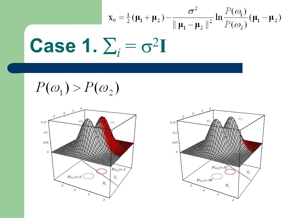
Case 1. i = 2 I irrelevant

49
Case 1. i = 2 I

50
Boundary btw. i and j

51
Case 1. i = 2 I Boundary btw. i and j wTwT w x0x0 x xx0xx0 The decision boundary will be a hyperplane perpendicular to the line btw. the means at somewhere. 0 if P ( i )= P ( j ) midpoint
= P ( j ) midpoint.")
52
Case 1. i = 2 I Minimum distance classifier (template matching)
")
53
Case 1. i = 2 I

55
Demo

56
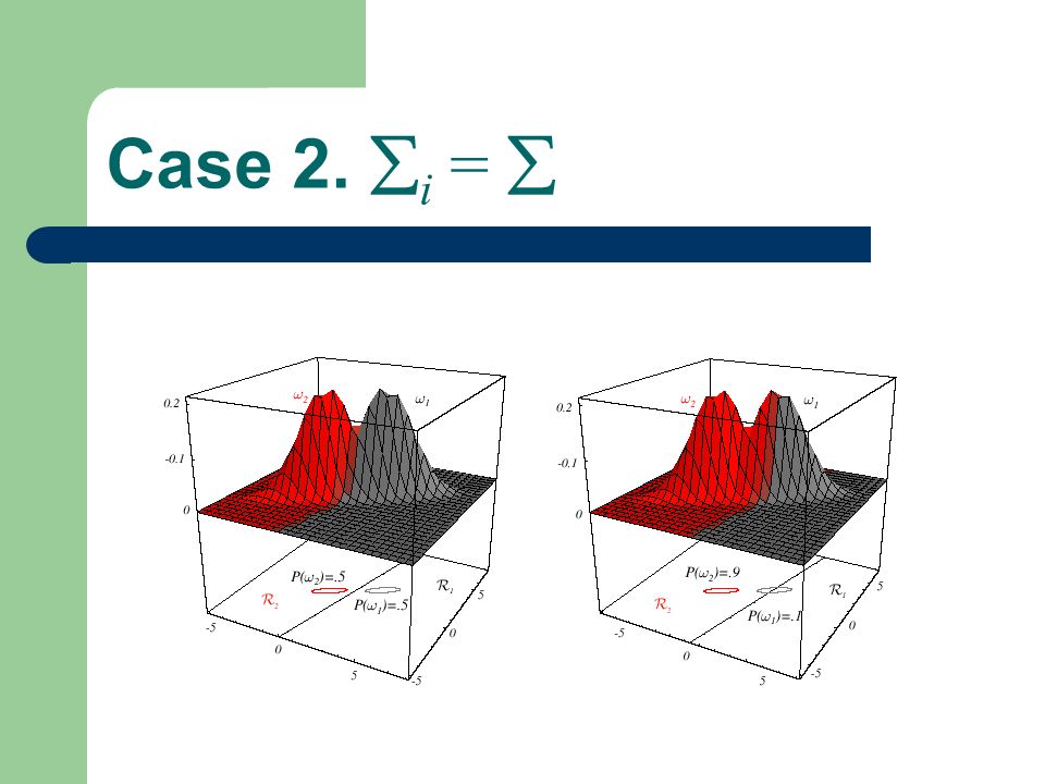
Case 2. i = Irrelevant if P ( i )= P ( j ) i, j Mahalanobis Distance irrelevant
= P ( j ) i, j Mahalanobis Distance irrelevant")
57
Case 2. i = Irrelevant

58
Case 2. i = w x0x0 x

60
Demo

61
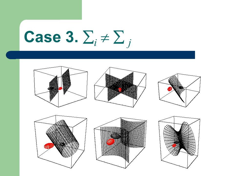
Case 3. i j irrelevant Without this term In Case 1 and 2 Decision surfaces are hyperquadrics, e.g., hyperplanes hyperspheres hyperellipsoids hyperhyperboloids

62
Case 3. i j Non-simply connected decision regions can arise in one dimensions for Gaussians having unequal variance.

63
Case 3. i j

65
Demo

66
Multi-Category Classification

67
Bayesian Decision Theory (Classification) Minimax Criterion
 Minimax Criterion")
68
Bayesian Decision Rule: Two-Category Classification Decide 1 if Likelihood Ratio Threshold Minimax criterion deals with the case that the prior probabilities are unknown.

69
Basic Concept on Minimax To choose the worst-case prior probabilities (the maximum loss) and, then, pick the decision rule that will minimize the overall risk. Minimize the maximum possible overall risk.

70
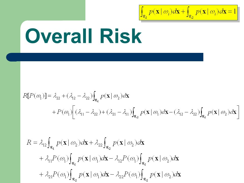
Overall Risk

74
The overall risk for a particular P( 1 ). The value depends on the setting of decision boundary The value depends on the setting of decision boundary R(x) = ax + b
 = ax + b.")
75
Overall Risk = 0 for minimax solution = R mm, minimax risk R(x) = ax + b Independent on the value of P( i ).
 = ax + b Independent on the value of P( i ).")
76
Minimax Risk

77
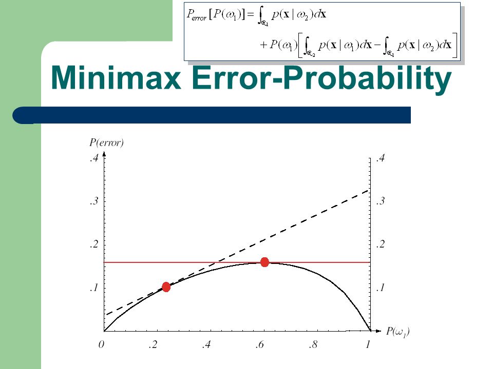
Error Probability Use 0/1 loss function

78
Minimax Error-Probability Use 0/1 loss function P(1|2)P(1|2) P(2|1)P(2|1)
P(1|2) P(2|1)P(2|1)")
79
Minimax Error-Probability R1R1 R2R2 11 22 P(1|2)P(1|2) P(2|1)P(2|1)
P(1|2) P(2|1)P(2|1)")
81
Bayesian Decision Theory (Classification) Neyman-Pearson Criterion
 Neyman-Pearson Criterion")
82
Bayesian Decision Rule: Two-Category Classification Decide 1 if Likelihood Ratio Threshold Neyman-Pearson Criterion deals with the case that both loss functions and the prior probabilities are unknown.

83
Signal Detection Theory The theory of signal detection theory evolved from the development of communications and radar equipment the first half of the last century. It migrated to psychology, initially as part of sensation and perception, in the 50's and 60's as an attempt to understand some of the features of human behavior when detecting very faint stimuli that were not being explained by traditional theories of thresholds.

84
The situation of interest A person is faced with a stimulus (signal) that is very faint or confusing. The person must make a decision, is the signal there or not. What makes this situation confusing and difficult is the presences of other mess that is similar to the signal. Let us call this mess noise.

85
Example Noise is present both in the environment and in the sensory system of the observer. The observer reacts to the momentary total activation of the sensory system, which fluctuates from moment to moment, as well as responding to environmental stimuli, which may include a signal.

86
Example A radiologist is examining a CT scan, looking for evidence of a tumor. A Hard job, because there is always some uncertainty. There are four possible outcomes: – hit (tumor present and doctor says "yes'') – miss (tumor present and doctor says "no'') – false alarm (tumor absent and doctor says "yes") – correct rejection (tumor absent and doctor says "no"). Two types of Error
 – miss (tumor present and doctor says no ) – false alarm (tumor absent and doctor says yes ) – correct rejection (tumor absent and doctor says no ). Two types of Error.")
87
Correct Rejection The Four Cases P(1|1)P(1|1) Miss False Alarms Hit Signal (tumor) Absent ( 1 ) Present ( 2 ) Decision No ( 1 ) Yes ( 2 ) P(2|2)P(2|2) P(1|2)P(1|2) P(2|1)P(2|1) Signal detection theory was developed to help us understand how a continuous and ambiguous signal can lead to a binary yes/no decision.
P(1|1) Miss False Alarms Hit Signal (tumor) Absent ( 1 ) Present ( 2 ) Decision No ( 1 ) Yes ( 2 ) P(2|2)P(2|2) P(1|2)P(1|2) P(2|1)P(2|1) Signal detection theory was developed to help us understand how a continuous and ambiguous signal can lead to a binary yes/no decision.")
88
No ( 1 ) Yes ( 2 ) Decision Making d’d’ Noise 11 Noise + Signal 22 Criterion Hit False Alarm Discriminability Based on expectancy (decision bias) P(2|2)P(2|2) P(2|1)P(2|1)
 Yes ( 2 ) Decision Making d’d’ Noise 11 Noise + Signal 22 Criterion Hit False Alarm Discriminability Based on expectancy (decision bias) P(2|2)P(2|2) P(2|1)P(2|1)")
89
ROC Curve (Receiver Operating Characteristic) Hit False Alarm P H =P( 2 | 2 ) P FA =P( 2 | 1 )
 Hit False Alarm P H =P( 2 | 2 ) P FA =P( 2 | 1 )")
90
Neyman-Pearson Criterion False Alarm P FA =P( 2 | 1 ) NP: max. P H subject to P FA ≦ a Hit P H =P( 2 | 2 )
.")
91
Likelihood Ratio Test where T is a threshold that meets the P FA constraint ( ≦ a). How to determine T?

92
Likelihood Ratio Test PHPH P FA R2R2 R1R1

93
Neyman-Pearson Lemma Consider the aforementioned rule with T chosen to give P FA ( ) = a. There is no decision rule ’ such that P FA ( ’ ) a and P H ( ’ ) > P H ( ). Pf) Let ’ be a decision rule with =1 0 0 > 0> 0
 a and P H ( ’ ) > P H ( ). Pf) Let ’ be a decision rule with =1 0 0 > 0> 0.")
94
Neyman-Pearson Lemma Consider the aforementioned rule with T chosen to give P FA ( ) = a. There is no decision rule ’ such that P FA ( ’ ) ≦ a and P H ( ’ ) > P H ( ). Pf) Let ’ be a decision rule with =0 00 00
 ≦ a and P H ( ’ ) > P H ( ). Pf) Let ’ be a decision rule with =0 00 00 .")
95
OK Neyman-Pearson Lemma Consider the aforementioned rule with T chosen to give P FA ( ) = a. There is no decision rule ’ such that P FA ( ’ ) ≦ a and P H ( ’ ) > P H ( ). Pf) Let ’ be a decision rule with 00
 ≦ a and P H ( ’ ) > P H ( ). Pf) Let ’ be a decision rule with 00.")
Similar presentations


 Minimum-Error-Rate Classification Classifiers, Discriminant Functions and Decision Surfaces The Normal Density.>")
 0 Pattern Classification All materials in these slides were taken from Pattern Classification (2nd ed) by R.>")
: Bayesian Decision Theory (Sections 2.1-2.2) Introduction Bayesian Decision Theory–Continuous Features.>")
 0 Pattern Classification All materials in these slides were taken from Pattern Classification (2nd ed) by R.>")
 Minimum-Error-Rate Classification Classifiers, Discriminant Functions and Decision Surfaces The Normal Density.>")
0 Pattern Classification All materials in these slides were taken from Pattern Classification (2nd ed) by R. O.>")


 by R. O. Duda, P. E. Hart and D. G. Stork, John Wiley.>")
 – Sections>")

 by R. O. Duda, P. E. Hart and D. G. Stork, John.>")
 Introduction Bayesian Decision Theory–Continuous Features All materials used in this course were taken from.>")

 Bayesian Decision Theory Discriminant Functions for the Normal Density Bayes Decision Theory – Discrete Features All materials used.>")
