1. NARROW-BAND FREQUENCY MODULATION
For small values of ,
Thus the expression for FM signal

2. can be expanded as
since
Then
since

3. Amplitude spectrum (single-sided plot)

4. WIDE-BAND FREQUENCY MODULATION
Wide-band FM signal.
In order to compute the spectrum of an angle-modulated signal with a sinusoidal message signal, let
Where q(t) = Phase deviation

5. The corresponding FM signal is given by
It may alternatively be written as
where Re(x) denotes the real part of x.

6. The parameter  is known as the modulation index and is the maximum value of phase deviation of the FM signal.
Consider the function z(t) given by
It is periodic with frequency fm and can therefore be expanded in a Fourier series as follows.

7. The Fourier coefficient are given by

8. Hence we can rewrite cn as
The integral on the right hand side is a function of “n” and  and is known as the Bessel function of the first kind of order n and argument .

9. It is conventionally denoted by Jn(  ). That is,
Thus
we get

10. x(t) is accordingly given by
The discrete spectrum of x(t) is, therefore, given by

11. PROPERTIES OF BESSEL FUNCTIONS
Property - 1:
For n even,
we have Jn () = J-n ()
For n odd,
we have Jn () = (-1) J-n ()
Thus,
Jn () = (-1)n J-n ()

12. Property - 2:
For small values of the modulation index 
we have
J0 ()  1
J1 ()  /2
J3 ()  0 for n > 2
Property - 3:

13. TABLE OF BESSEL FUNCTIONS

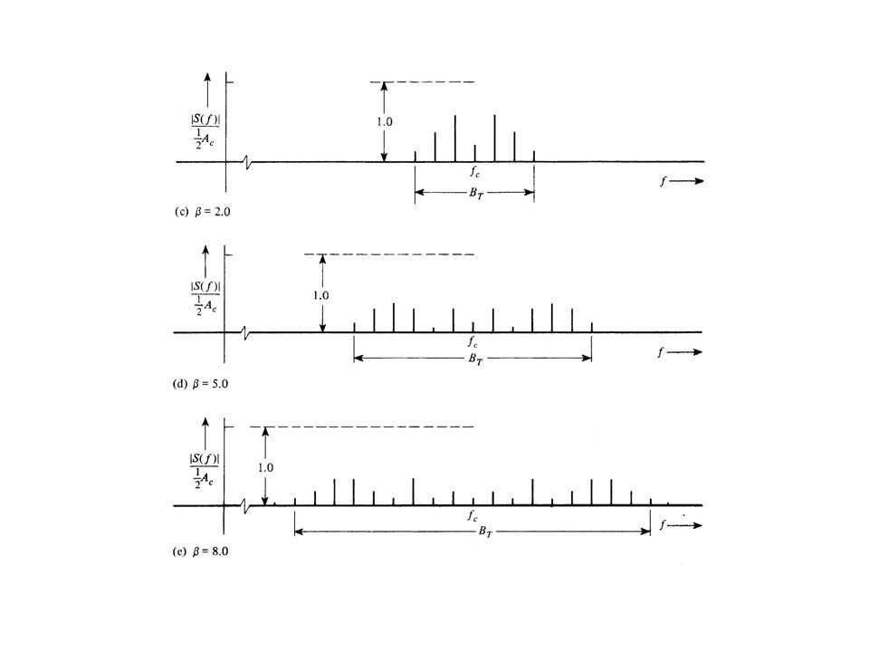
14. AMPLITUDE SPECTRUM

16. With the increase in the modulation index, the carrier amplitude decreases while the amplitude of the various sidebands increases. With some values of modulation index, the carrier can disappear completely.

17. POWER IN ANGLE-MODULATED SIGNAL
The power in an angle-modulated signal is easily computed

18. Thus the power contained in the FM signal is independent of the message signal. This is an important difference between FM and AM.
The time-average power of an FM signal may also be obtained from

19. where

20. TRANSMISSION BANDWIDTH OF FM SIGNALS
Theoretically, a FM signal contains an infinite number of side frequencies so that the bandwidth required to transmit such signal is infinite.
However, since the values of Jn() become negligible for sufficiently large n, the bandwidth of an angle-modulated signal can be defined by considering only those terms that contain significant power.

21. In practice, the bandwidth of a FM signal can be determined by knowing the modulation index and using the Bessel function table.

22. Example:
Determine bandwidth with table of bessel functions
Calculate the bandwidth occupied by a FM signal with a modulation index of 2 and a highest modulating frequency of 2.5 kHz.

23. Referring to the table, we can see that this produces six significant pairs of sidebands. The bandwidth can then be determined with the simple formula
where N is the number of significant sidebands.

24. Using the example above and assuming a highest modulating frequency of 2.5 kHz, the bandwidth of the FM signal is

25. DETERMINE BW WITH CARSON'S RULE
An alternative way to calculate the bandwidth of a FM signal is to use Carson's rule. This rule takes into consideration only the power in the most significant sidebands whose amplitudes are greater than 2 percent of the carrier. These are the sidebands whose values are 0.02 or more.

26. Carson's rule is given by the expression
In this expression, f is the maximum frequency deviation, and fm is the maximum modulating frequency.

27. We may thus define an approximate rule for the transmission bandwidth of an FM signal generated by a single of frequency fm as follows:

28. Example:
Assuming a maximum frequency deviation of 5 kHz and a maximum modulating frequency of 2.5 kHz, the bandwidth would be

29. Comparing the bandwidth with that computed in the preceding example, you can see that Carson's rule gives a smaller bandwidth.

30. FM SIGNAL GENERATION
They are two basic methods of generating frequency-Modulated signals
Direct Method
Indirect Method

31. DIRECT FM
In a direct FM system the instantaneous frequency is directly varied with the information signal. To vary the frequency of the carrier is to use an Oscillator whose resonant frequency is determined by components that can be varied. The oscillator frequency is thus changed by the modulating signal amplitude.

32. For example, an electronic Oscillator has an output frequency that depends on energy-storage devices. There are a wide variety of oscillators whose frequencies depend on a particular capacitor value. By varying the capacitor value, the frequency of oscillation varies. If the capacitor variations are controlled by m(t), the result is an FM waveform

33. INDIRECT FM

34. Angle modulation includes frequency modulation FM and phase modulation PM.
FM and PM are interrelated; one cannot change without the other changing. The information signal frequency also deviates the carrier frequency in PM.
Phase modulation produces frequency modulation. Since the amount of phase shift is varying, the effect is that, as if the frequency is changed.

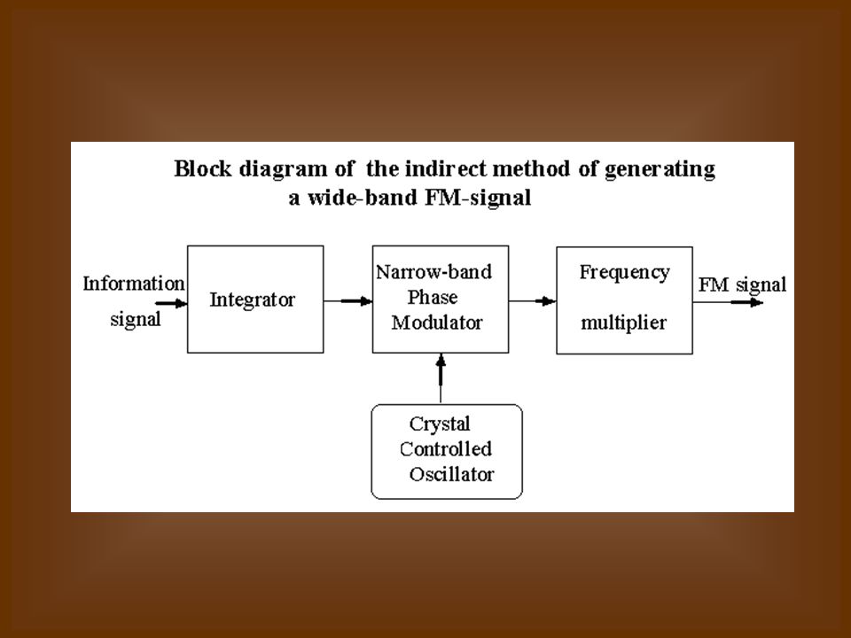
35. Since FM is produced by PM , the later is referred to as indirect FM.
The information signal is first integrated and then used to phase modulate a crystal-controlled oscillator, which provides frequency stability.
In order to minimize the distortion in the phase modulator, the modulation index is kept small, thereby is resulting in a narrow-band FM-signal

36. The narrow-band FM signal is multiplied in frequency by means of frequency multiplier so as to produce the desired wide-band FM signal.
The frequency multiplier is used to perform narrow band to wideband conversion.
The frequency deviation of this new waveform is “M” times that of the old, while the rate at which the instantaneous frequency varies has not changed