Download presentation
Presentation is loading. Please wait.

1
A. Yu. Smirnov International Centre for Theoretical Physics, Trieste, Italy Institute for Nuclear Research, RAS, Moscow, Russia E. Akhmedov, M. Maltoni, A.S., JHEP 0705:077 (2007) ; arXiv:0804.1466 (hep-ph) JHEP (2008) A.S. hep-ph/0610198.
 ; arXiv: (hep-ph) JHEP (2008) A.S. hep-ph/")
2
inner core outer core upper mantle transition zone crust lower mantle (phase transitions in silicate minerals) liquid solid Fe Si PREM model A.M. Dziewonski D.L Anderson 1981 R e = 6371 km

3
core mantle flavor to flavor transitions Oscillations in multilayer medium - nadir angle core-crossing trajectory -zenith angle = 33 o accelerator atmospheric cosmic neutrinos Applications:

4
P. Lipari, M. Chizhov, M. Maris, S.Petcov T. Ohlsson T. Kajita e Contours of constant oscillation probability in energy- nadir (or zenith) angle plane Michele Maltoni
 angle plane Michele Maltoni.")
5
from SAND to HAND Explaining oscillograms Dependence of oscillograms on neutrino parameters Applications CP-violation domains What these oscillograms for? Neutrino images of the earth 6X2

7
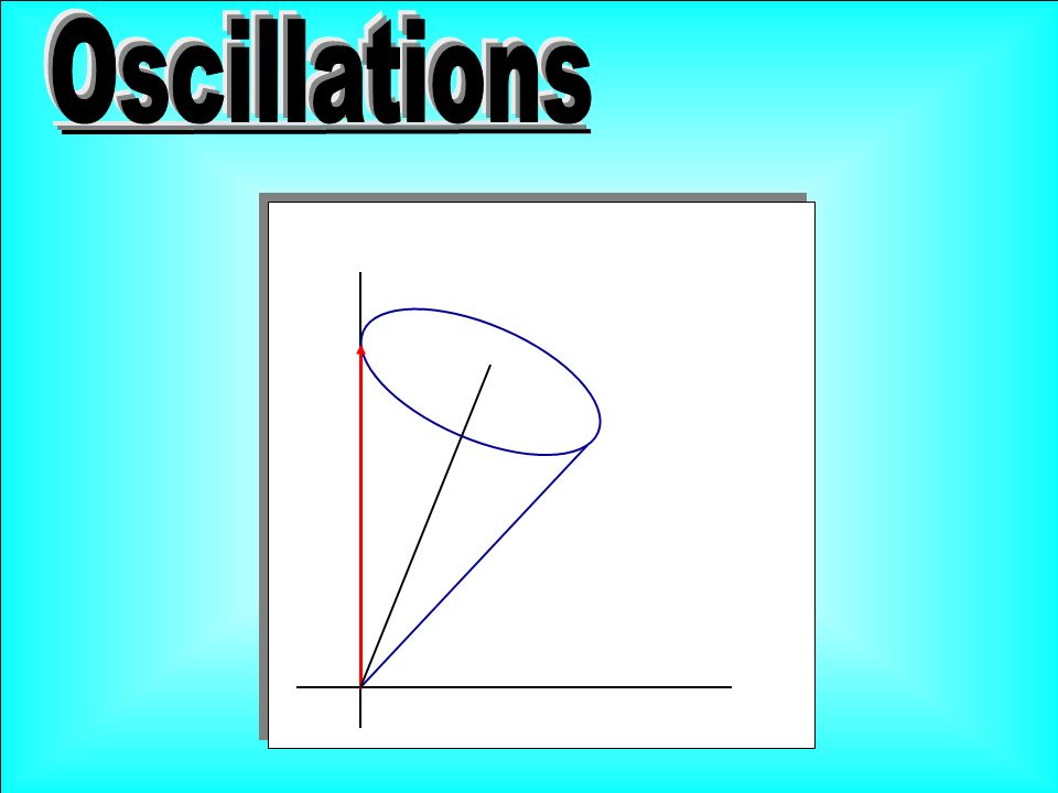
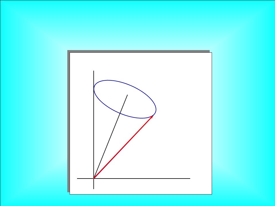
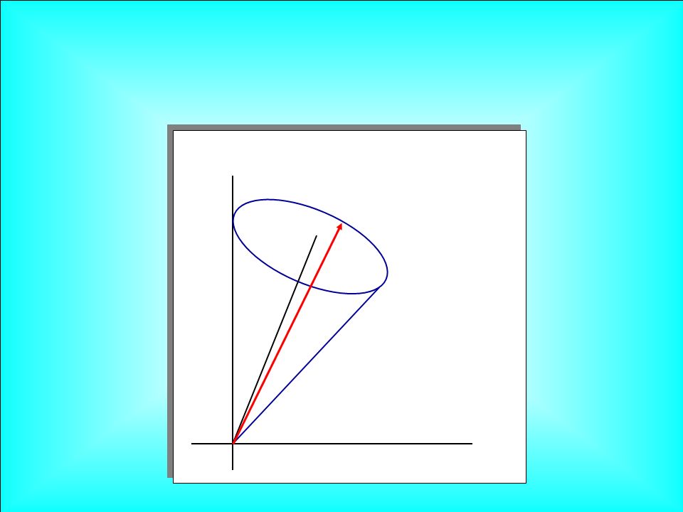
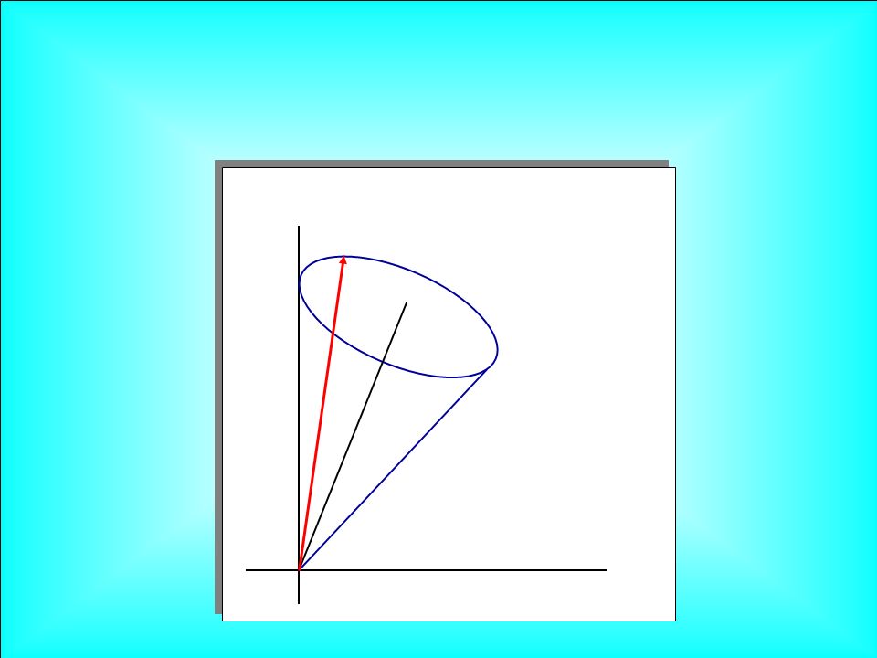
Re e + , P = Im e + , e + e - 1/2 B = (sin 2 , 0, cos2 ) = ( B x P ) d P dt Coincides with equation for the electron spin precession in the magnetic field = e , Polarization vector: P = + Evolution equation: i = H d d t d d t i = (B ) Differentiating P and using equation of motion m 2 /2E
 = ( B x P ) d P dt Coincides with equation for the electron spin precession in the magnetic field = e , Polarization vector: P = + Evolution equation: i = H d d t d d t i = (B ) Differentiating P and using equation of motion m 2 /2E")
8
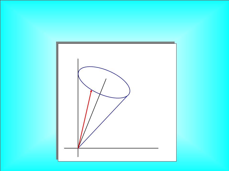
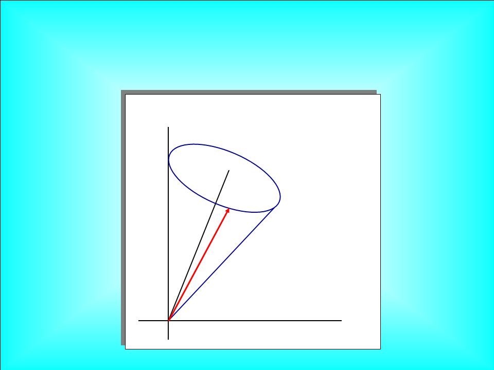
= P = (Re e + , Im e + , e + e - 1/2) B = (sin 2 m, 0, cos2 m ) 2 l m = ( B x ) d dt Evolution equation = 2 t/ l m - phase of oscillations P = e + e = Z + 1/2 = cos 2 Z /2 probability to find e e ,
 B = (sin 2 m, 0, cos2 m ) 2 l m = ( B x ) d dt Evolution equation = 2 t/ l m - phase of oscillations P = e + e = Z + 1/2 = cos 2 Z /2 probability to find e e ,")
15
Oscillations in matter with nearly constant density Parametric enhancement of oscillations (mantle - core – - mantle) (mantle) Interference constant density + corrections Peaks due to resonance enhancement of oscillations Low energies: adiabatic approximation Parametric resonance parametric peaks Smallness of 13 and m 21 2 / m 32 2 in the first approximation: overlap of two 2 –patterns due to 1-2 and 1-3 mixings interference of modes CP-interference interference (sub-leading effect) Qiu-Yu Liu, A.S.
 (mantle) Interference constant density + corrections Peaks due to resonance enhancement of oscillations Low energies: adiabatic approximation Parametric resonance parametric peaks Smallness of 13 and m 21 2 / m 32 2 in the first approximation: overlap of two 2 –patterns due to 1-2 and 1-3 mixings interference of modes CP-interference interference (sub-leading effect) Qiu-Yu Liu, A.S.")
16
MSW-resonance peaks 1-2 mixing 1 - P ee Parametric peak 1-2 mixing MSW-resonance peak, 1-3 mixing Parametric ridges 1-3 mixing MSW-resonance peak, 1-3 mixing

17
mantle 1 2 12

18
core mantle mantle core mantle 1 2 3 4 1 2 3 4

19
core mantle 1 2 3 4 3 2 4 1

20
determine localizations of the peaks and ridges Generalized resonance condition Intersection of the corresponding lines determines positions of the peaks phase: = + k depth: sin2 m = 1 Generalizations of the conditions ``AMPLITUDE = 1’’ in matter with constant density to the case of 1 or 3 layers with varying densities also determine position of other features: minima, saddle points, etc

21
generalized phase condition collinearity condition Maximal oscillation effects: Amplitude (resonance) condition Phase condition Generalizations: E.Kh. Akhmedov; M. Chizhov S. Petcov

23
Dependence on neutrino parameters and earth density profile (tomography)
")
24
Flow of large probability toward larger Lines of flow change weakly Factorization of 13 dependence Position of the mantle MSW peak measurement of 13

25
normal inverted neutrino antineutrino For 2 system

27
Under CP-transformations: c CP- transformations: c = i 0 2 + applying to the chiral components U PMNS U PMNS * - V - V usual medium is C-asymmetric which leads to CP asymmetry of interactions

28
= 60 o Standard parameterization

29
= 130 o

30
= 315 o

31
Three grids of lines: Solar magic lines Atmospheric magic lines Interference phase lines

32
e e f U 23 I I = diag (1, 1, e i ) e e S ~ Propagation basis ~ ~ ~ ~ projection propagation A( e ) = cos 23 A e2 e i + sin 23 A e3 A e3 A e2
 e e S ~ Propagation basis ~ ~ ~ ~ projection propagation A( e ) = cos 23 A e2 e i + sin 23 A e3 A e3 A e2")
33
P( e ) = |cos 23 A e2 e i + sin 23 A e3 | 2 ``atmospheric’’ amplitude``solar’’ amplitude Due to specific form of matter potential matrix (only V ee = 0) dependence on and 23 is explicit P( e ) = |A e2 A e3 | cos ( - ) P( ) = - |A e2 A e3 | cos cos P( ) = - |A e2 A e3 | sin sin For maximal 2-3 mixing = arg (A e2 * A e3 ) = 0
 = |cos 23 A e2 e i + sin 23 A e3 | 2 ``atmospheric’’ amplitude``solar’’ amplitude Due to specific form of matter potential matrix (only V ee = 0) dependence on and 23 is explicit P( e ) = |A e2 A e3 | cos ( - ) P( ) = - |A e2 A e3 | cos cos P( ) = - |A e2 A e3 | sin sin For maximal 2-3 mixing = arg (A e2 * A e3 ) = 0")
34
A e2 ~ A S ( m 21 2, 12 ) A e3 ~ A S ( m 31 2, 13 ) are not valid in whole energy range due to the level crossing S ~ H 21 S ~ m 32 2 A ~ H 32 corrections of the order m 12 2 / m 13 , s 13 2 A S ~ i sin2 12 m sin L l 12 m A A ~ i sin2 13 m sin L l 13 m For constant density:
 A e3 ~ A S ( m 31 2, 13 ) are not valid in whole energy range due to the level crossing S ~ H 21 S ~ m 32 2 A ~ H 32 corrections of the order m 12 2 / m 13 , s 13 2 A S ~ i sin2 12 m sin L l 12 m A A ~ i sin2 13 m sin L l 13 m For constant density:")
35
P( e ) = c 23 2 |A S | 2 + s 23 2 |A A | 2 + 2 s 23 c 23 |A S | |A A | cos( + ) L l ij m at high energies: l 12 m ~ l 0 L = k l 0, k = 1, 2, 3 A S = 0 for (for three layers – more complicated condition) s 23 = sin 23 = arg (A S A A *) Dependence on disappears if Solar ``magic’’ lines does not depend on energy - magic baseline V. Barger, D. Marfatia, K Whisnant P. Huber, W. Winter, A.S. A S = 0 A A = 0 Atmospheric magic lines L = k l 13 m (E), k = 1, 2, 3, … = k
, k = 1, 2, 3, … = k .")
36
A S = 0 - true value of phase f - fit value P = P( ) - P( f ) P = 0 (along the magic lines) ( + ) = - ( + f ) + 2 k (E, L) = - ( + f )/2 + k = P int ( ) - P int ( f ) A A = 0 int. phase condition depends on How to measure the interference term? Interference term: P = 2 s 23 c 23 |A S | |A A | [ cos( + ) - cos ( + f )] For e channel:
 - cos ( + f )] For e channel:.")
37
A S = 0 P = 0 (along the magic lines) = /2 + k A A = 0 interference phase does not depends on P( ) ~ - 2 s 23 c 23 |A S | |A A | cos cos For channel - dependent part: The survival probabilities is CP-even functions of No CP-violation. P ~ 2 s 23 c 23 |A S | |A A | cos [cos - cos f ] P( ) ~ - 2 s 23 c 23 |A S | |A A | sin sin
 ~ - 2 s 23 c 23 |A S | |A A | sin sin .")
38
solar magic lines atmospheric magic lines relative phase lines Regions of different sign of P Interconnection of lines due to level crossing factorization is not valid

39
Grid (domains) does not change with Int. phase line moves with -change PP
 does not change with Int. phase line moves with -change PP")
40
PP

41
PP

42
Contour plots for the probability difference P = P max – P min for varying between 0 – 360 o e E min ~ 0.57 E R E min 0.5 E R when 13 0

44
- mass hierarchy - 1-3 mixing - CP violation Pictures for Textbooks: neutrino images of the Earth

45
10 1 100 0.1 E, GeV MINOS T2K CNGS NuFac 2800 0.005 0.03 0.10 T2KK Degeneracy of parameters Large atmospheric neutrino detectors LAND LENF

46
Intense and controlled beams Small effect Degeneracy of parameters Combination of results from different experiments is in general required Cover poor-structure regions Systematic errors Small fluxes, with uncertainties Large effects Cover rich-structure regions No degeneracy?

47
E ~ 0.1 – 10 4 GeV Problem: - small statistics - uncertainties in the predicted fluxes - presence of several fluxes - averaging and smoothing effects Cost-free source whole range of nadir anglesL ~ 10 – 10 4 km Several neutrino types - various flavors: e and - neutrinos and antineutrinos Cover whole parameter space (E, )
")
48
INO – Indian Neutrino observatory HyperKamiokande Y. Suzuki.. Icecube (1000 Mton) 50 kton iron calorimenter 0.5 Megaton water Cherenkov detectors Underwater detectors ANTARES, NEMO TITAND (Totally Immersible Tank Assaying Nuclear Decay) 2 Mt and more UNO E > 30 – 50 GeV Reducing down 20 GeV?
 50 kton iron calorimenter 0.5 Megaton water Cherenkov detectors Underwater detectors ANTARES, NEMO TITAND (Totally Immersible Tank Assaying Nuclear Decay) 2 Mt and more UNO E > 30 – 50 GeV Reducing down 20 GeV .")
49
Y. Suzuki - Proton decay searches - Supernova neutrinos - Solar neutrinos Totally Immersible Tank Assaying Nucleon Decay TITAND-II: 2 modules: 4.4 Mt (200 SK) Under sea deeper than 100 m Cost of 1 module 420 M $ Modular structure
 Under sea deeper than 100 m Cost of 1 module 420 M $ Modular structure.")
50
e-like events - angular resolution: ~ 3 o - neutrino direction: ~ 10 o - energy resolution for E > 4 GeV better than 2% E/E = [0.6 + 2.6 E/GeV ] % cos -1 / -0.8 -0.8 / -0.6 -0.6 / -0.4 2.5 – 5 GeV SR 2760 (10) 3320 (20) 3680 (15) MR 2680 (9) 2980 (12) 3780 (13) Fully contained events 5 – 10 GeV SR 1050 (9) 1080 (5) 1500 (10) MR 1150 (4) 1280 (3) 1690 (6) SR – single ring MR – multi-ring (…) – number of events detected by 4SK years MC: 800 SK-years zenith angle
![e-like events - angular resolution: ~ 3 o - neutrino direction: ~ 10 o - energy resolution for E > 4 GeV better than 2% E/E = [ E/GeV ] % cos -1 / / / – 5 GeV SR 2760 (10) 3320 (20) 3680 (15) MR 2680 (9) 2980 (12) 3780 (13) Fully contained events 5 – 10 GeV SR 1050 (9) 1080 (5) 1500 (10) MR 1150 (4) 1280 (3) 1690 (6) SR – single ring MR – multi-ring (…) – number of events detected by 4SK years MC: 800 SK-years zenith angle](http://images.slideplayer.com/26/8488269/slides/slide_50.jpg "e-like events - angular resolution: ~ 3 o - neutrino direction: ~ 10 o - energy resolution for E > 4 GeV better than 2% E/E = [ E/GeV ] % cos -1 / / / – 5 GeV SR 2760 (10) 3320 (20) 3680 (15) MR 2680 (9) 2980 (12) 3780 (13) Fully contained events 5 – 10 GeV SR 1050 (9) 1080 (5) 1500 (10) MR 1150 (4) 1280 (3) 1690 (6) SR – single ring MR – multi-ring (…) – number of events detected by 4SK years MC: 800 SK-years zenith angle")
51
2 = 2 [N – N 0 + N 0 log N 0 /N] N = P F N 0 = N( m 21 2 = 0, = 0)- zero sub-leading effects For atmospheric neutrinos Poisson e
![ 2 = 2 [N – N 0 + N 0 log N 0 /N] N = P F N 0 = N( m 21 2 = 0, = 0)- zero sub-leading effects For atmospheric neutrinos Poisson e ](http://images.slideplayer.com/26/8488269/slides/slide_51.jpg " 2 = 2 [N – N 0 + N 0 log N 0 /N] N = P F N 0 = N( m 21 2 = 0, = 0)- zero sub-leading effects For atmospheric neutrinos Poisson e ")
52
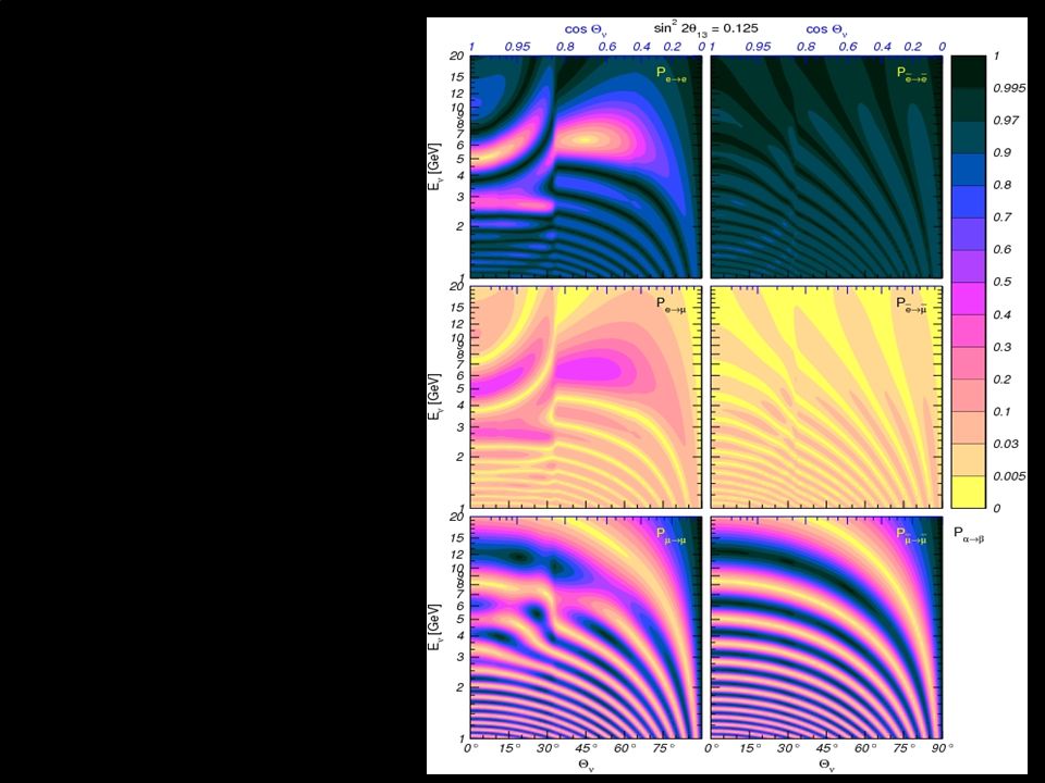
Lines of equal 2 sin 2 2 = 0.125 No averaging

53
smoothing

54
Measuring oscillograms with atmospheric neutrinos E > 2 - 3 GeV with sensitivity to the resonance region Huge Atmospheric Neutrino Detector Better angular and energy resolution Spacing of PMT ? V = 5 - 10 MGt Should we reconsider a possibility to use atmospheric neutrinos? develop new techniques to detect atmospheric neutrinos with low threshold in huge volumes? 0.5 GeV

55
Oscillograms encode in a comprehensive way information about the Earth matter profile and neutrino oscillation parameters. Oscillograms have specific dependencies on 1-3 mixing angle, mass hierarchy, CP-violating phases and earth density profile that allows us to disentangle their effects. CP-effect has a domain structure. The borders of domains are determined by three grids of lines: the solar magic lines, the atmospheric magic lines and the lines of interference phase condition Locations of salient structures of oscillograms are determined by the collinearity and generalized phase conditions Determination of neutrino parameters,tomography by measuring oscillograms with Huge (multi Megaton) atmospheric neutrino detectors?
 atmospheric neutrino detectors .")
56
P( e ) = |cos 23 A S e i + sin 23 A A | 2 |A S | ~ sin2 12 m sin L l m For high energiesl m l 0 for trajectory with L = l 0 A S = 0 P = |sin 23 A A | 2 no dependence on For three layers – more complicated condition Magic trajectories associated to A A = 0 ``atmospheric’’ amplitude ``solar’’ amplitude mainly, m 13 2, 13 mainly, m 12 2, 12 Contours of suppressed CP violation effects
 = |cos 23 A S e i + sin 23 A A | 2 |A S | ~ sin2 12 m sin L l m For high energiesl m l 0 for trajectory with L = l 0 A S = 0 P = |sin 23 A A | 2 no dependence on For three layers – more complicated condition Magic trajectories associated to A A = 0 ``atmospheric’’ amplitude ``solar’’ amplitude mainly, m 13 2, 13 mainly, m 12 2, 12 Contours of suppressed CP violation effects")
57
1 layer: MSW resonance condition S (1) 11 = S (1) 22 Im (S 11 S 12 *) = 0 Im S (1) 11 = 0 sin = 0cos 2 m = 0 2 layers: X 3 = 0S (2) 11 = S (2) 22 Im S (2) 11 = 0 Generalized resonance condition valid for both cases: = + k Re S (1) 11 = 0 another representation: For symmetric profile (T –invariance): Re (S 11 ) = 0 Im S 11 = 0 Parametric resonance condition unitarity: S (1) 11 = [S (1) 22 ]* S 12 - imaginary
![1 layer: MSW resonance condition S (1) 11 = S (1) 22 Im (S 11 S 12 *) = 0 Im S (1) 11 = 0 sin = 0cos 2 m = 0 2 layers: X 3 = 0S (2) 11 = S (2) 22 Im S (2) 11 = 0 Generalized resonance condition valid for both cases: = + k Re S (1) 11 = 0 another representation: For symmetric profile (T –invariance): Re (S 11 ) = 0 Im S 11 = 0 Parametric resonance condition unitarity: S (1) 11 = [S (1) 22 ]* S 12 - imaginary](http://images.slideplayer.com/26/8488269/slides/slide_57.jpg "1 layer: MSW resonance condition S (1) 11 = S (1) 22 Im (S 11 S 12 *) = 0 Im S (1) 11 = 0 sin = 0cos 2 m = 0 2 layers: X 3 = 0S (2) 11 = S (2) 22 Im S (2) 11 = 0 Generalized resonance condition valid for both cases: = + k Re S (1) 11 = 0 another representation: For symmetric profile (T –invariance): Re (S 11 ) = 0 Im S 11 = 0 Parametric resonance condition unitarity: S (1) 11 = [S (1) 22 ]* S 12 - imaginary")
58
S = a b -b* a* Evolution matrix for one layer (2 -mixing): a, b – amplitudes of probabilities For symmetric profile (T-invariance) b = - b* For two layers:S (2) = S 1 S 2 A = S (2) 12 = a 2 b 1 + b 2 a 1 * transition amplitude: The amplitude is potentially maximal if both terms have the same phase (collinear in the complex space): arg (a 1 a 2 b 1 ) = arg (b 2 ) Due to symmetry of the core Re b 2 = 0 Re (a 1 a 2 b 1 ) = 0 Due to symmetry of whole profile it gives extrema condition for 3 layers Re b = 0 Another way to generalize parametric resonance condition from unitarity condition
: a, b – amplitudes of probabilities For symmetric profile (T-invariance) b = - b* For two layers:S (2) = S 1 S 2 A = S (2) 12 = a 2 b 1 + b 2 a 1 * transition amplitude: The amplitude is potentially maximal if both terms have the same phase (collinear in the complex space): arg (a 1 a 2 b 1 ) = arg (b 2 ) Due to symmetry of the core Re b 2 = 0 Re (a 1 a 2 b 1 ) = 0 Due to symmetry of whole profile it gives extrema condition for 3 layers Re b = 0 Another way to generalize parametric resonance condition from unitarity condition")
59
Different structures follow from different realizations of the collinearity and phase condition in the non-constant case. Re (a 1 a 2 b 1 ) = 0 X 3 = 0 P = 1 Re (S 11 ) = 0 Absolute maximum (mantle, ridge A) c 1 = 0, c 2 = 0 s 1 = 0, c 2 = 0 Local maxima Core-enhancement effect P = sin (4 m – 2 c ) Saddle points at low energies Maxima at high energies above resonances
 = 0 X 3 = 0 P = 1 Re (S 11 ) = 0 Absolute maximum (mantle, ridge A) c 1 = 0, c 2 = 0 s 1 = 0, c 2 = 0 Local maxima Core-enhancement effect P = sin (4 m – 2 c ) Saddle points at low energies Maxima at high energies above resonances.")
60
P( e a ) = sin 2 2 m sin 2 L l m Oscillation Probability constant density Amplitude of oscillations half-phase oscillatory factor - mixing angle in matter l m (E, n ) m (E, n ) – oscillation length in matter Conditions for maximal transition probability: P = 1 1. Amplitude condition: sin 2 2 m = 1 2. Phase condition: = + k MSW resonance condition m m l m l In vacuum: l m = 2 /(H 2 – H 1 )
.")
61
1.Take condition for constant density Generalization of the amplitude and phase conditions to varying density case 2. Write in terms of evolution matrix 3. Apply to varying density This generalization leads to new realizations which did not contained in the original condition; more physics content S 11 S 12 S 21 S 22 S(x) = T exp - i H dx = x 0
 = T exp - i H dx = x 0.")
62
l = 4 m 2 Oscillation length in vacuum Refraction length l 0 = 2 2 G F n e - determines the phase produced by interaction with matter lmlm E l0l0 ERER Resonance energy: l (E R ) = l 0 cos2 l /sin2 l = l 0 /cos2 ) (maximum at ~ l 2 H 2 - H 1 l m =
 = l 0 cos2 l /sin2 l = l 0 /cos2 ) (maximum at ~ l 2 H 2 - H 1 l m =")
63
Simulations: Monte Carlo simulations for SK 100 SK year scaled to 800 SK-years (18 Mtyr) = 4 years of TITAND-II Assuming normal mass hierarchy: Sensitivity to quadrant: sin 2 23 = 0.45 and 0.55 can be resolved with 99% C.L. (independently of value of 1-3 mixing) Sensitivity to CP-violation: down to sin 2 2 13 = 0.025 can be measured with = 45 o accuracy ( 99% CL)
 Sensitivity to CP-violation: down to sin 2 2 13 = can be measured with = 45 o accuracy ( 99% CL).")
64
a). Resonance in the mantle b). Resonance in the core c). Parametric ridge A d). Parametric ridge B e). Parametric ridge C f). Saddle point a). b). c). e). d). f).
. Parametric ridge B e). Parametric ridge C f). Saddle point a). b). c). e). d). f)..")
65
Contour plots for the probability difference P = P max – P min for varying between 0 – 360 o Averaging?

66
Enhancement associated to certain conditions for the phase of oscillations Another way of getting strong transition No large vacuum mixing and no matter enhancement of mixing or resonance conversion ``Castle wall profile’’ V = = V. Ermilova V. Tsarev, V. Chechin E. Akhmedov P. Krastev, A.S., Q. Y. Liu, S.T. Petcov, M. Chizhov 1 2 3 4 5 6 7 mm mm m m

67
of oscillograms 1. One (or zero) MSW peak in the mantle domain 2. Three parametric peaks (ridges) in the core domain 3. MSW peak in the core domain 1-3 mixing: 1-2 mixing: Depending on value of sin 2 13 1. Three MSW peaks in the mantle domain 2. One (or 2) parametric peak (ridges) in the core domain 1D 2D - structuresregular behavior
 in the core domain 3. MSW peak in the core domain 1-3 mixing: 1-2 mixing: Depending on value of sin 2 Three MSW peaks in the mantle domain 2. One (or 2) parametric peak (ridges) in the core domain 1D 2D - structuresregular behavior.")
68
Y. Suzuki Totally Immersible Tank Assaying Nucleon Decay Module: - 4 units, one unit: tank 85m X 85 m X 105 m - mass of module 3 Mt, fiducial volume 2.2 Mt - photosensors 20% coverage ( 179200 50 cm PMT) TITAND-II: 2 modules: 4.4 Mt (200 SK)
 TITAND-II: 2 modules: 4.4 Mt (200 SK).")
71
Contours of constant oscillation probability in energy- nadir (or zenith) angle plane P. Lipari, T. Ohlsson M. Chizhov, M. Maris, S.Petcov T. Kajita e Michele Maltoni 1 - P ee

Similar presentations


 Atmospheric Solar –SNO & SK-I Active solar –SK.>")

 田 (da) 義 (yoshi) 章 (aki) with Lin Guey-Lin ( 林 貴林 ) National Chiao-Tung University.>")


 for Super-Kamiokande Collaboration December 9, RCCN International Workshop Effect of solar terms to 23 determination in.>")
>")

