1. Numerical Models for Geophysical Fluid Dynamics Applications: Do we really need more new models?* Frank Giraldo Department of Applied Mathematics Naval Postgraduate School, Monterey CA USA http://faculty.nps.edu/fxgirald Collaborators: Matthias Läuter (AWI, Potsdam), Marco Restelli (Max-Planck, Hamburg), Emil Constantinescu (Argonne NL, Chicago), Jim Kelly (NPS) *Funded by the Office of Naval Research: (1) Computational Mathematics and (2) Meteorology

2. The Answer is Yes! But we need to answer why. Numerical models are used in GFD to study the atmosphere and ocean, mostly separately but recently interest in coupled modeling has increased. However, numerous models already exist so why do we need to develop more models? Here are a few reasons for considering new models: 1.Computer architectures change – this affects the efficiency of an existing model. So, we must design the numerical method to take full advantage of the computing platform (e.g., global vs. local methods). 2.Increased computational power – with more computational power comes more resolution (more grid points in your model). This has immediate consequences in the validity of some assumptions in your governing equations of motion (e.g., hydrostatic vs. non-hydrostatic). 3.Variability of models is important for ensembles; this is important for NWP (e.g., tropical cyclone tracking) but is this important for climate? I would be interested in such a discussion. 4.New numerics should give us increased capabilities. However, the numerics of the dynamics is not sufficient to give us better results. We also need to revisit the methodologies used within the physical parameterizations. The models are only as good as their weakest links (e.g., dynamics, physics, initial conditions, boundary conditions).

3. Talk Summary Part I 1.How do computer architectures affect the models? Vector versus Distributed-memory computers Global versus Local Methods 2.Can Local Methods compete with Global Methods? Accuracy and Efficiency 3.How does resolution affect the models? Hydrostatic versus Non-hydrostatic models and regions of validity of the governing equations 4.How can we systematically improve the Physical Parameterizations Hierarchy of simple to complex representations Part II  Results of a new storm-surge model under development Currently, we only have tsunami wave propagation

4. 1. How do computer architectures affect Models?

5. Domain Decomposition: How does one break-up the problem across processors? Global Method: N proc = O(T) Local Method: N proc =O(T 2 )

6. Communication: What information do processors require? Global Method: All-to-all communication stencil Local Method: Small communication stencil

7. Operation Count Local Method (e.g., NSEAM, ICON) –O(T 2 N N lev ) quadratic dependence on resolution Global Method (e.g., IFS, GFS, ECHAM, NOGAPS) –O(T 3 N lev ) cubic dependence on resolution Local Method Proof: –The total cost is O(n H 2 N 3 N lev ) –Now, let T= n H N which then gives O(T 2 N N lev ) Global Method Proof: –The total cost is O( N lat 3 N lev + N lon log N lon N lev ) –Now, let T= 2/3 N lat which gives O(T 3 N lev )

8. 2. Can Local Methods compete with Global Methods?

9. NSEAM T72 L20 (Local Method) Zonal mean zonal wind averaged using the last 1000 days of the simulation. Both models yield very similar results where the mid-latitude jets are clearly visible in both models. Accuracy of Global and Local Methods (Held-Suarez Test run for 1200 days) IFS T106 L30 (Global Method)

10. Accuracy of a Local Method (Surface Values for T185 L26 during 0-30 days) Pressure Temperature 30 day simulation for a fully 3D atmospheric model for the Jablonowski-Williamson Baroclinic Instability problem

11. Jablonowski-Williamson Baroclinic Instability NASA is the Lin-Rood model (finite volume semi-Lagrangian), GME is the DWD model (finite volume) model, and NCAR is the community climate model (spherical harmonics). NASA and GME (dashed lines) are 2 nd order models while NCAR and NSEAM are high-order models. NSEAM and NCAR behave similarly.

12. Advantages of Local Methods: Adaptive Unstructured Grid Capabilities Unfortunately, not all local methods allow for such flexibility. Only if the model is built directly on top of triangles can this flexibility be used. ICON, NSEAM, and the new model being developed at AWI-Potsdam and NPS are such models.

13. Icosahedral Telescoping Hexahedral Icosahedral Adaptive Geometric Flexibility of Local Methods Adaptive Quadrilaterals Triangles Banded

14. Performance of Global versus Local Methods (T239 L30 DT=300 seconds) Local Global

15. Scalability of Local Methods IBM SP4 (1.7 GHz) Note that the problem size from T249 L30 to T498 L60 has increased by a factor of 16 (2 2 hor x 2 vert x 2 time-steps). However, the Wallclock Time has only decreased by a factor of 8. Furthermore, NSEAM T498 L60 scales linearly with processor count! At T498 L60 NSEAM can theoretically accommodate 70,000 processors! T249 (54 km) L30 DT=300 secs T498 (20 km) L60 DT=150 secs

16. 3. How does resolution affect the Models?

17. Non-hydrostatic Equations (fully compressible Euler equations) (Mass) (Momentum) (Energy) (Equation of State )

18. Non-hydrostatic Equations (Expanded Form) (Mass) (H-Momentum) (Energy) (Equation of State ) (V-Momentum) (W-Momentum)

19. Hydrostatic Equations (Mass) (H-Momentum) (Energy) (Equation of State ) (V-Momentum) (W-Momentum)

20. Pseudo-Incompressible Equations (Very Similar to the Compressible equations) (Mass) (H-Momentum) (Energy) (Equation of State ) (V-Momentum) (W-Momentum)

21. When are these equations valid? 1.Non-hydrostatic Equations These equations are valid at all spatial scales; these are the most general form of the governing equations. The problem with this form is that they permit acoustic waves which are very fast and have little effects on the dynamical processes we are interested in. We know how to solve these equations well but requires sophisticated numerical methods (DG, semi-implicit, etc.) 2.Hydrostatic Equations These are very simple equations to solve but are not valid if you are interested in vertical acceleration. Because vertical acceleration is omitted, it then means that the vertically propagating acoustic waves are removed from the equations. This approximation is no longer valid below 10km resolution. Many NWP models are either at this limit or approaching it quickly (e.g., IFS, UM, Grapes). 3.Pseudo-Incompressible Equations It would be nice to keep the equations valid below 10km without having to deal with the vertically propagating acoustic waves; these equations are a likely candidate. No operational NWP or climate models currently use this approach, only research codes (e.g., EULAG). It would be interesting to explore this form of the equations (joint work with R. Klein and M. Läuter).

22. 4. How can we systematically improve the physical parameterization?

23. How can we improve the Parameterizations? Like with the dynamics, we need a hierarchy of levels of complexity. E.g., for dyamics, we have: 1.Shallow Water equations on the Sphere 2.Hydrostatic/Non-hydrostatic equations in x-z 3.Hydrostatic equations in 3D (e.g., NSEAM) 4.Non-hydrostatic equations in 3D and on the sphere (under development with M. Läuter). We need the same thing for the physical parameterization. I am only aware of the following hierarchy of complexity: 1.Dry dynamics with simple solar forcing (Held-Suarez) 2.Dynamics with Kessler physics (2 or 3 phases of moisture) 3.Dynamics with full physics but with no terrain and prescribed SST (Aqua- Planet) The simplest of these (excluding Held-Suarez) are already quite complex and so it is difficult to discern what should the correct model behavior be. More work needs to be done in this area and we need people well-versed in physics to work with numerical analysts to build better physics that takes advantage of the new dynamical cores.

24. NSEAM T72 L20 (Local Method) Zonal mean zonal wind averaged using the last 1000 days of the simulation. Both models yield very similar results where the mid-latitude jets are clearly visible in both models. Held-Suarez Test (A good test, but a very simple one) IFS T106 L30 (Global Method)

25. Nonhydrostatic Model with Kessler Physics (3 phases of water: vapor, condensation, precip) Vapor Rain Clouds This test is already quite complicated and requires very careful analysis to discern whether or not the model behaves correctly.

26. Control Control Day 0~180 Surface Temperature & Convective Precipitation Aqua-Planet Experiments (~T54)

27. Control 3.75° x 2.5° L19 Neale & Hoskins (2001) 1800W0E 0180180ControlControl Convective Precipitation (-5°~5°) NSEAM E6P8L20 (~2.2°~T54) UKMO Tomita NICAM Cloud Resolving Model 1800W0E w/ reduced Hyperviscosity (  =5e5)

28. Part I: Summary We believe we have a good handle on the governing equations of motion and how to solve them accurately and efficiently on big computers However, in order to take full advantage of these new equations, methods, and computers requires a better coupling of the dynamics and physics. The physics is responsible for the skill of a forecast and so there needs to be as much time spent on this aspect as on dynamical cores and numerical methods for these. In order to construct a “new physics” requires a step-by-step construction and integration of the physics into dynamical cores so that both the atmospheric physicist and the applied mathematician both understand how best to construct and validate the new codes. We need a hierarchy of physical parameterizations from simple to very complex in order to fully understand and improve the models. It has been my experience that physics has been constructed as a collection of various codes (implemented by different people and at different places). This makes it very difficult to understand how all of these processes work together. In contrast, dynamical cores, data assimilation, and normal mode initialization routines are always written by the same persons. IPAM Meeting Next March-June: Model and Data Hierarchies for Simulating and Understanding Climate www.ipam.ucla.edu/programs/cl2010

29. Part II: Some results of a new storm-surge model under development

30. (Copyright Anders Grawin, 2006) Coastal Ocean Model Collaborators: D. Alevras (Hellenic Hydrography Lab), J. Behrens (U. Hamburg), T. Warburton (Rice), M. Restelli (U. Sevilla),

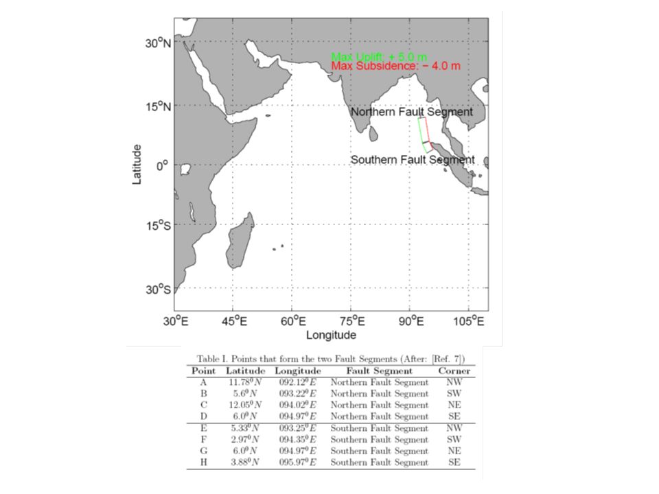
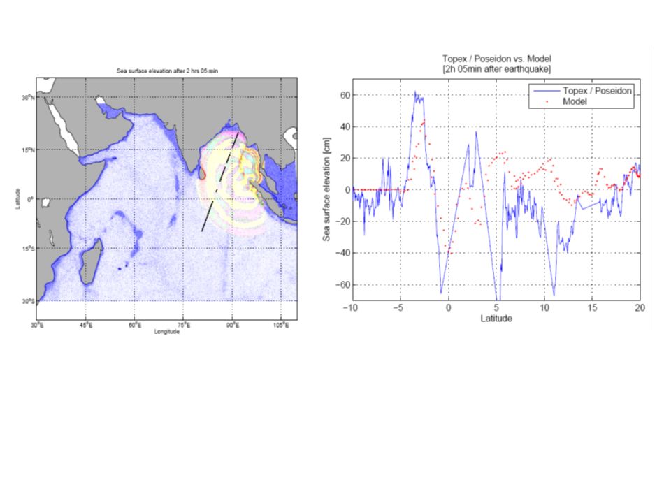
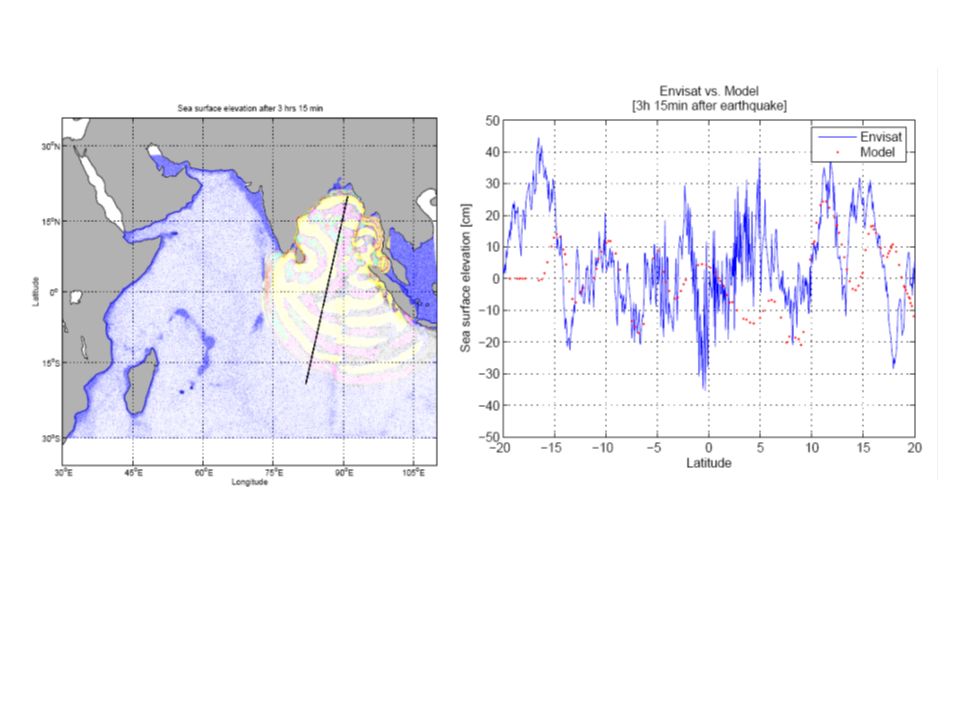
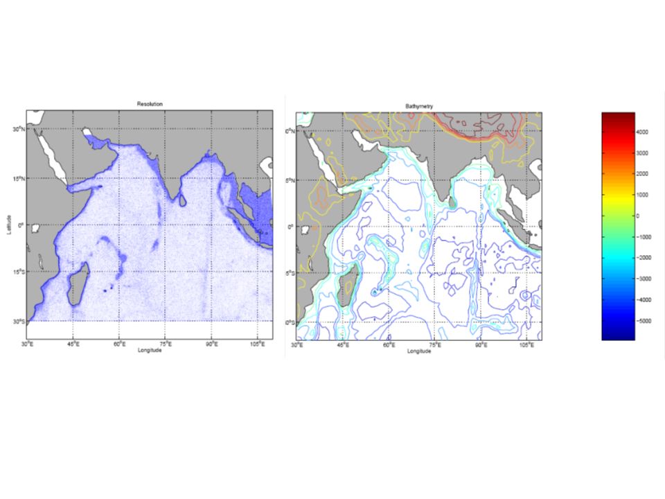
31. Propagation of the 2004 Indian Ocean Tsunami (Grid Dimensions: Np=66715, Ne=130444, N=1, K=2, J=1) Time evolution of the water surface height x y

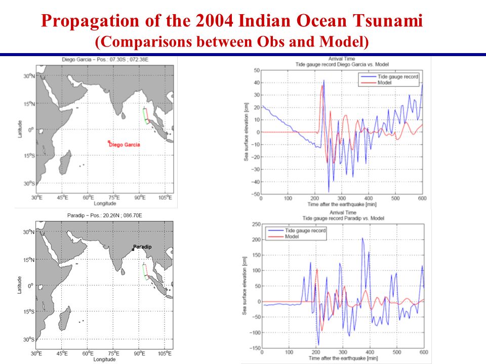
33. Black color: National Institute of Oceanography (NIO), Goa, India http://www.nio.org/datainfo/tidegauge.html Red color : University of Hawaii's Sea Level Center database (Honolulu) http://ilikai.soest.hawaii.edu/uhslc/iot1d/index.html Blue color: "Mercator" depth gauge recording of 26 December 2004 tsunami http://www.knmi.nl

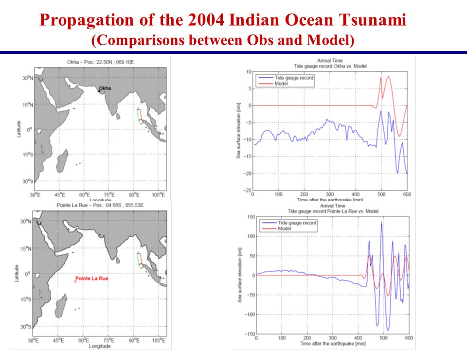
34. Propagation of the 2004 Indian Ocean Tsunami (Comparisons between Obs and Model) y

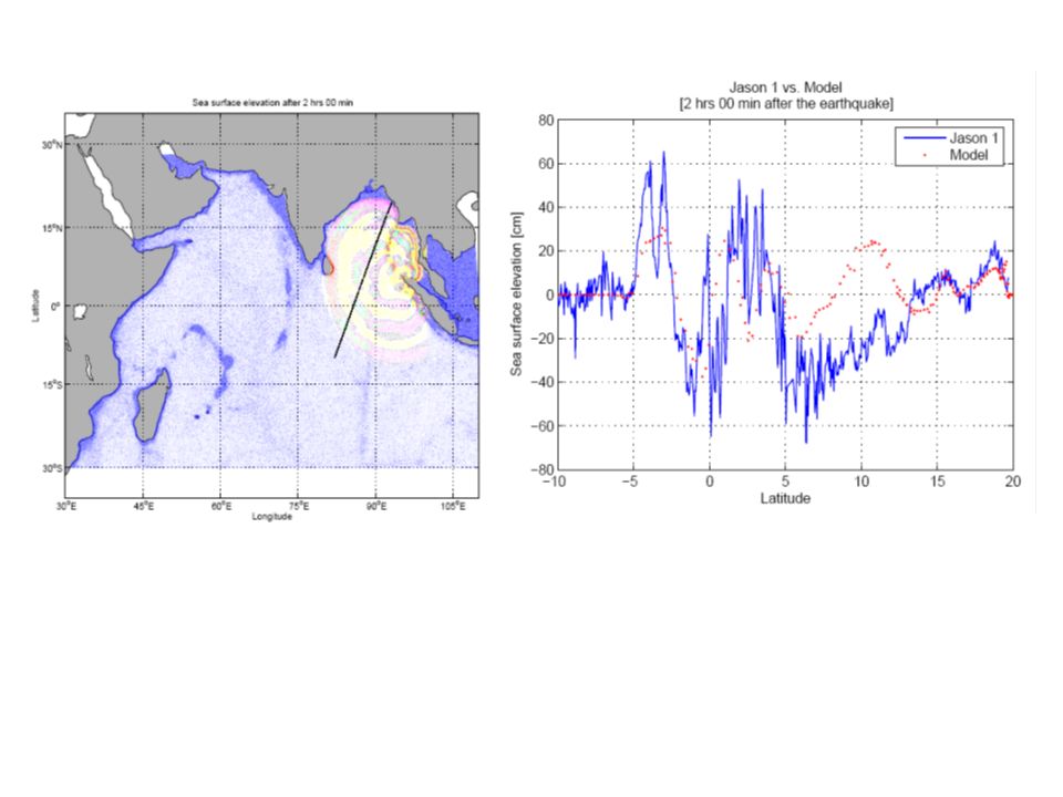
38. Black color: TOPEX / POSEIDON 2 hrs 05 min Red color : Jason 1 2 hrs 00 min Green color: Envisat 3 hrs 15 min NOAA (http://nctr.pmel.noaa.gov/indo1204.html)http://nctr.pmel.noaa.gov/indo1204.html