Download presentation
Presentation is loading. Please wait.

1
776 Computer Vision Jan-Michael Frahm, Enrique Dunn Spring 2013

2
No class Tuesday Feb 12 th Faculty candidate Wed, Feb 13 th, 4 pm, SN011

3
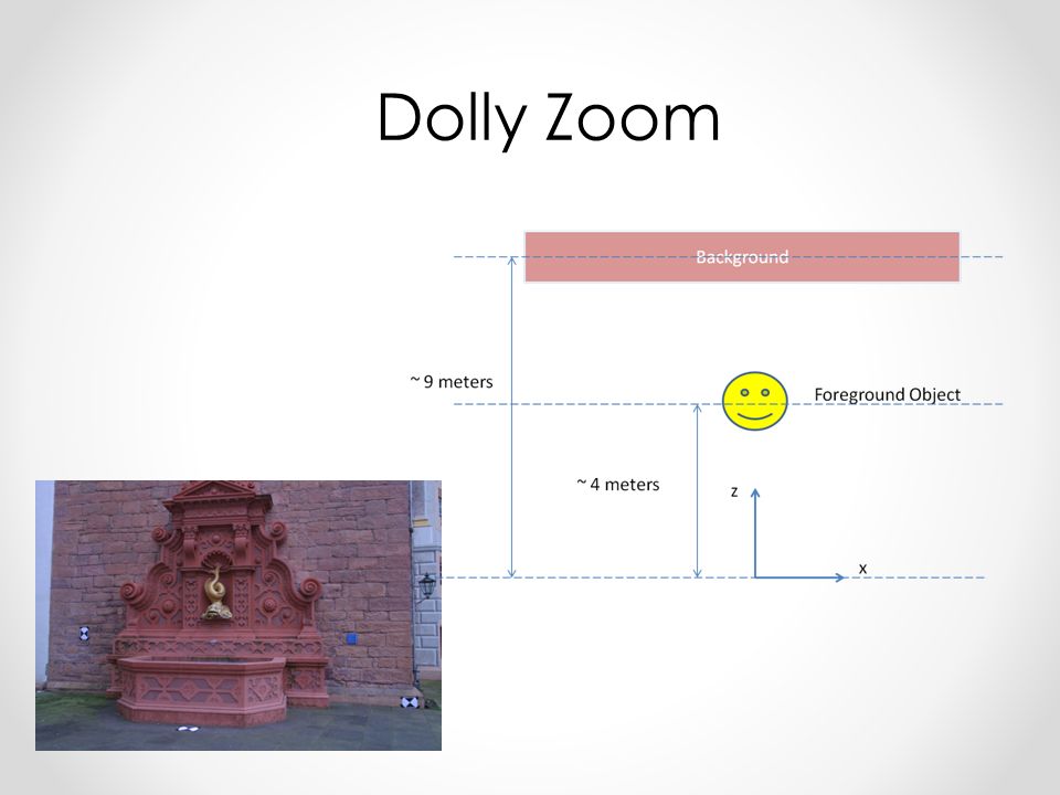
www.cs.unc.edu/~jmf/teaching/spring2013/2Assignm ent776-Spring2013.pdf Dolly Zoom

5
Sample Dolly Zoom Video

6
Radial Distortion

7
Brown’s distortion model o accounts for radial distortion o accounts for tangential distortion (distortion caused by lens placement errors) typically K 1 is used or K 1, K 2, K 3, P 1, P 2 (x u, y u ) undistorted image point as in ideal pinhole camera (x d,y d ) distorted image point of camera with radial distortion (x c,y c ) distortion center K n n-th radial distortion coefficient P n n-th tangential distortion coefficient
 typically K 1 is used or K 1, K 2, K 3, P 1, P 2 (x u, y u ) undistorted image point as in ideal pinhole camera (x d,y d ) distorted image point of camera with radial distortion (x c,y c ) distortion center K n n-th radial distortion coefficient P n n-th tangential distortion coefficient")
9
Last Class There are two principled ways for finding correspondences: 1.Matching o Independent detection of features in each frame o Correspondence search over detected features +Extends to large transformations between images -High error rate for correspondences 2.Tracking o Detect features in one frame o Retrieve same features in the next frame by searching for equivalent feature (tracking) +Very precise correspondences +High percentage of correct correspondences -Only works for small changes in between frames
 +Very precise correspondences +High percentage of correct correspondences -Only works for small changes in between frames")
10
Fitting Least squares Total least squares

11
Distance between point (x i, y i ) and line ax+by=d (a 2 +b 2 =1): |ax i + by i – d| Find (a, b, d) to minimize the sum of squared perpendicular distances (x i, y i ) ax+by=d Unit normal: N=(a, b) Solution to ( U T U)N = 0, subject to ||N|| 2 = 1 : eigenvector of U T U associated with the smallest eigenvalue (least squares solution to homogeneous linear system UN = 0 )
 and line ax+by=d (a 2 +b 2 =1): |ax i + by i – d| Find (a, b, d) to minimize the sum of squared perpendicular distances (x i, y i ) ax+by=d Unit normal: N=(a, b) Solution to ( U T U)N = 0, subject to ||N|| 2 = 1 : eigenvector of U T U associated with the smallest eigenvalue (least squares solution to homogeneous linear system UN = 0 )")
13
RANSAC Robust fitting can deal with a few outliers – what if we have very many? Random sample consensus (RANSAC): Very general framework for model fitting in the presence of outliers Outline o Choose a small subset of points uniformly at random o Fit a model to that subset o Find all remaining points that are “close” to the model and reject the rest as outliers o Do this many times and choose the best model M. A. Fischler, R. C. Bolles. Random Sample Consensus: A Paradigm for Model Fitting with Applications to Image Analysis and Automated Cartography. Comm. of the ACM, Vol 24, pp 381-395, 1981.Random Sample Consensus: A Paradigm for Model Fitting with Applications to Image Analysis and Automated Cartography
: Very general framework for model fitting in the presence of outliers Outline o Choose a small subset of points uniformly at random o Fit a model to that subset o Find all remaining points that are close to the model and reject the rest as outliers o Do this many times and choose the best model M. A. Fischler, R. C. Bolles. Random Sample Consensus: A Paradigm for Model Fitting with Applications to Image Analysis and Automated Cartography. Comm. of the ACM, Vol 24, pp , 1981.Random Sample Consensus: A Paradigm for Model Fitting with Applications to Image Analysis and Automated Cartography.")
14
RANSAC for line fitting example

15
Least-squares fit

16
RANSAC for line fitting example 1.Randomly select minimal subset of points

17
RANSAC for line fitting example 1.Randomly select minimal subset of points 2.Hypothesize a model

18
RANSAC for line fitting example 1.Randomly select minimal subset of points 2.Hypothesize a model 3.Compute error function Source: R. Raguram

19
RANSAC for line fitting example 1.Randomly select minimal subset of points 2.Hypothesize a model 3.Compute error function 4.Select points consistent with model

20
RANSAC for line fitting example 1.Randomly select minimal subset of points 2.Hypothesize a model 3.Compute error function 4.Select points consistent with model 5.Repeat hypothesize-and- verify loop

21
21 RANSAC for line fitting example 1.Randomly select minimal subset of points 2.Hypothesize a model 3.Compute error function 4.Select points consistent with model 5.Repeat hypothesize-and- verify loop

22
22 RANSAC for line fitting example 1.Randomly select minimal subset of points 2.Hypothesize a model 3.Compute error function 4.Select points consistent with model 5.Repeat hypothesize-and- verify loop Uncontaminated sample

23
RANSAC for line fitting example 1.Randomly select minimal subset of points 2.Hypothesize a model 3.Compute error function 4.Select points consistent with model 5.Repeat hypothesize-and- verify loop

24
RANSAC for line fitting Repeat N times: Draw s points uniformly at random Fit line to these s points Find inliers to this line among the remaining points (i.e., points whose distance from the line is less than t ) If there are d or more inliers, accept the line and refit using all inliers
 If there are d or more inliers, accept the line and refit using all inliers")
25
Choosing the parameters Initial number of points s o Typically minimum number needed to fit the model Distance threshold t o Choose t so probability for inlier is p (e.g. 0.95) o Zero-mean Gaussian noise with std. dev. σ: t 2 =3.84σ 2 Number of samples N o Choose N so that, with probability p, at least one random sample is free from outliers (e.g. p=0.99) (outlier ratio: e)
 o Zero-mean Gaussian noise with std. dev. σ: t 2 =3.84σ 2 Number of samples N o Choose N so that, with probability p, at least one random sample is free from outliers (e.g. p=0.99) (outlier ratio: e).")
26
Choosing the parameters Initial number of points s o Typically minimum number needed to fit the model Distance threshold t o Choose t so probability for inlier is p (e.g. 0.95) o Zero-mean Gaussian noise with std. dev. σ: t 2 =3.84σ 2 Number of samples N o Choose N so that, with probability p, at least one random sample is free from outliers (e.g. p=0.99) (outlier ratio: e) proportion of outliers e s5%10%20%25%30%40%50% 2235671117 33479111935 435913173472 54612172657146 64716243797293 748203354163588 8592644782721177
 o Zero-mean Gaussian noise with std. dev. σ: t 2 =3.84σ 2 Number of samples N o Choose N so that, with probability p, at least one random sample is free from outliers (e.g. p=0.99) (outlier ratio: e) proportion of outliers e s5%10%20%25%30%40%50%")
27
Choosing the parameters Initial number of points s o Typically minimum number needed to fit the model Distance threshold t o Choose t so probability for inlier is p (e.g. 0.95) o Zero-mean Gaussian noise with std. dev. σ: t 2 =3.84σ 2 Number of samples N o Choose N so that, with probability p, at least one random sample is free from outliers (e.g. p=0.99) (outlier ratio: e)
 o Zero-mean Gaussian noise with std. dev. σ: t 2 =3.84σ 2 Number of samples N o Choose N so that, with probability p, at least one random sample is free from outliers (e.g. p=0.99) (outlier ratio: e).")
28
Choosing the parameters Initial number of points s o Typically minimum number needed to fit the model Distance threshold t o Choose t so probability for inlier is p (e.g. 0.95) o Zero-mean Gaussian noise with std. dev. σ: t 2 =3.84σ 2 Number of samples N o Choose N so that, with probability p, at least one random sample is free from outliers (e.g. p=0.99) (outlier ratio: e) Consensus set size d o Should match expected inlier ratio
 o Zero-mean Gaussian noise with std. dev. σ: t 2 =3.84σ 2 Number of samples N o Choose N so that, with probability p, at least one random sample is free from outliers (e.g. p=0.99) (outlier ratio: e) Consensus set size d o Should match expected inlier ratio.")
29
Adaptively determining the number of samples Inlier ratio e is often unknown a priori, so pick worst case, e.g. 10%, and adapt if more inliers are found, e.g. 80% would yield e=0.2 Adaptive procedure: o N=∞, sample_count =0 o While N >sample_count Choose a sample and count the number of inliers Set e = 1 – (number of inliers)/(total number of points) Recompute N from e: Increment the sample_count by 1
/(total number of points) Recompute N from e: Increment the sample_count by 1.")
30
RANSAC pros and cons Pros o Simple and general o Applicable to many different problems o Often works well in practice Cons o Parameters to tune o Doesn’t work well for low inlier ratios (too many iterations, or can fail completely) o Can’t always get a good initialization of the model based on the minimum number of samples
 o Can’t always get a good initialization of the model based on the minimum number of samples")
31
Threshold free Robust Estimation Homography 1.Match points 2.Run RANSAC, threshold ≈ 1 - 2 pixels Common approach: Problem: Robust Estimation o Estimation of model parameters in the presence of noise and outliers

32
Motivation 1.Match points 2.Run RANSAC 3D similarity, threshold = ? 32

33
Motivation Robust estimation algorithms often require data and/or model specific threshold settings o Performance degrades when parameter settings deviate from the “true” values (Torr and Zisserman 2000, Choi and Medioni 2009) t = 0.01t = 0.001 t = 5.0 t = 0.5 33
 t = 0.01t = t = 5.0 t =")
34
Contributions Threshold-free robust estimation o No user-supplied inlier threshold o No assumption of inlier ratio o Simple, efficient algorithm 34

35
RECON Instead of per-model or point-based residual analysis We inspect pairs of models Inlier Outlier Sort points by distance to model “Inlier” models 35

36
RECON Instead of per-model or point-based residual analysis We inspect pairs of models Inlier Outlier “Outlier” models Sort points by distance to model 36

37
RECON Instead of per-model or point-based residual analysis We inspect pairs of models Inlier models Outlier models “Consistent” behaviour Random permutations of data points 37

38
RECON Instead of per-model or point-based residual analysis We inspect pairs of models “Happy families are all alike; every unhappy family is unhappy in its own way” - Leo Tolstoy, Anna Karenina Inlier models Outlier models “Consistent” behaviour Random permutations of data points 38

39
RECON Instead of per-model or point-based residual analysis We inspect pairs of models “Happy families are all alike; every unhappy family is unhappy in its own way” - Leo Tolstoy, Anna Karenina Inlier models “Consistent” behaviour Outlier models Random permutations of data points 39

40
RECON Instead of per-model or point-based residual analysis We inspect pairs of models “Consistent” behaviourRandom permutations of data points “Happy families are all alike; every unhappy family is unhappy in its own way” - Leo Tolstoy, Anna Karenina Outlier models Inlier models 40

41
How can we characterize this behaviour? Assuming that measurement error is GaussianRECON Inlier residuals are distributed If σ is known, can compute threshold t that finds some fraction α of all inliers Typically set to 0.95 or 0.99 Large overlap At the “true” threshold, inlier models capture a stable set of points t αIαI 41

42
How can we characterize this behaviour? What if σ is unknown? o Hypothesize values of noise scale σRECON t1t1 t2t2 t3t3 t4t4... tTtT t = ? 42

43
How can we characterize this behaviour? What if σ is unknown? o Hypothesize values of noise scale σRECON t θ t : fraction of common points θtθt t 43

44
How can we characterize this behaviour? What if σ is unknown? o Hypothesize values of noise scale σRECON θtθt θtθt θtθt θtθt θtθt θtθt θtθt θtθt θtθt θtθt θtθt θtθt θtθt t 44

45
At the “true” value of the threshold 1. A fraction ≈ α 2 of the inliers will be common to inlier modelsRECON θtθt θtθt θtθt θtθt θtθt θtθt θtθt θtθt θtθt θtθt θtθt θtθt θtθt α2α2 t 45

46
RECON θtθt t θtθt θtθt θtθt θtθt θtθt θtθt θtθt θtθt θtθt θtθt θtθt θtθt At the “true” value of the threshold 1. A fraction ≈ α 2 of the inliers will be common to inlier models 2. The inlier residuals correspond to the same underlying distribution 46

47
At the “true” value of the threshold 1. A fraction ≈ α 2 of the inliers will be common to inlier models 2. The inlier residuals correspond to the same underlying distributionRECON θtθt t Overlap is low at the true threshold Overlap can be high for a large overestimate of the noise scale Residuals are unlikely to correspond to the same underlying distribution Outlier models 47

48
At the “true” value of the threshold 1. A fraction ≈ α 2 of the inliers will be common to inlier models 2. The inlier residuals correspond to the same underlying distributionRECON 48

49
1. Hypothesis generation - Generate model M i from random minimal sample 2. Model evaluation - Compute and store residuals of M i to all data points 3. Test α – con sistency - For a pair of models M i and M j Check if overlap ≈ α 2 for some t Check if residuals come from the same distribution Residual Consensus: Algorithm Similar to RANSA C 49

50
1. Hypothesis generation - Generate model M i from random minimal sample 2. Model evaluation - Compute and store residuals of M i to all data points 3. Test α – con sistency - For a pair of models M i and M j Check if overlap ≈ α 2 for some t Check if residuals come from the same distribution Residual Consensus: Algorithm Find consistent pairs of models Efficient implementation: use residual ordering Single pass over sorted residuals 50

51
1. Hypothesis generation - Generate model M i from random minimal sample 2. Model evaluation - Compute and store residuals of M i to all data points 3. Test α – con sistency - For a pair of models M i and M j Check if overlap ≈ α 2 for some t Check if residuals come from the same distribution Residual Consensus: Algorithm Find consistent pairs of models Two-sample Kolmogorov-Smirnov test Reject null hypothesis at level β if 51

52
Residual Consensus: Algorithm 1. Hypothesis generation - Generate model M i from random minimal sample 2. Model evaluation - Compute and store residuals of M i to all data points 3. Test α – con sistency - For a pair of models M i and M j Check if overlap ≈ α 2 for some t Check if residuals come from the same distribution Repeat until K pairwise- consistent models are found 52

53
Residual Consensus: Algorithm 1. Hypothesis generation - Generate model M i from random minimal sample 2. Model evaluation - Compute and store residuals of M i to all data points 3. Test α – con sistency - For a pair of models M i and M j Check if overlap ≈ α 2 for some t Check if residuals come from the same distribution 4. Refine solution - Recompute final model and inliers 53 Repeat until K pairwise- consistent models are found

54
Experiments Real data 54

55
RECON Conclusion RECON is o Flexible: no data/model dependent threshold settings Inlier threshold Inlier ratio o Accurate: achieves results of the same quality as RANSAC without apriori knowledge of the noise parameters o Efficient: adapts to the inlier ratio in the data o Extensible: Can be combined with other RANSAC optimizations (non-uniform sampling, degeneracy handling, etc.) o Code: http://cs.unc.edu/~rraguram/recon
 o Code:")
56
Fitting: The Hough transform

57
Voting schemes Let each feature vote for all the models that are compatible with it Hopefully the noise features will not vote consistently for any single model Missing data doesn’t matter as long as there are enough features remaining to agree on a good model

58
Hough transform An early type of voting scheme General outline: o Discretize parameter space into bins o For each feature point in the image, put a vote in every bin in the parameter space that could have generated this point o Find bins that have the most votes P.V.C. Hough, Machine Analysis of Bubble Chamber Pictures, Proc. Int. Conf. High Energy Accelerators and Instrumentation, 1959 Image space Hough parameter space

59
Parameter space representation A line in the image corresponds to a point in Hough space Image spaceHough parameter space

60
Parameter space representation What does a point (x 0, y 0 ) in the image space map to in the Hough space? Image spaceHough parameter space

61
Parameter space representation What does a point (x 0, y 0 ) in the image space map to in the Hough space? o Answer: the solutions of b = –x 0 m + y 0 o This is a line in Hough space Image spaceHough parameter space

62
Parameter space representation Where is the line that contains both (x 0, y 0 ) and (x 1, y 1 )? Image spaceHough parameter space (x 0, y 0 ) (x 1, y 1 ) b = –x 1 m + y 1 Slide credit: S. Lazebnik
 (x 1, y 1 ) b = –x 1 m + y 1 Slide credit: S. Lazebnik.")
63
Parameter space representation Where is the line that contains both (x 0, y 0 ) and (x 1, y 1 )? o It is the intersection of the lines b = –x 0 m + y 0 and b = –x 1 m + y 1 Image spaceHough parameter space (x 0, y 0 ) (x 1, y 1 ) b = –x 1 m + y 1
 (x 1, y 1 ) b = –x 1 m + y 1.")
64
Problems with the (m,b) space: o Unbounded parameter domain o Vertical lines require infinite m Parameter space representation
 space: o Unbounded parameter domain o Vertical lines require infinite m Parameter space representation")
65
Problems with the (m,b) space: o Unbounded parameter domain o Vertical lines require infinite m Alternative: polar representation Parameter space representation Each point will add a sinusoid in the ( , ) parameter space
 space: o Unbounded parameter domain o Vertical lines require infinite m Alternative: polar representation Parameter space representation Each point will add a sinusoid in the ( , ) parameter space")
66
Algorithm outline Initialize accumulator H to all zeros For each edge point (x,y) in the image For θ = 0 to 180 ρ = x cos θ + y sin θ H(θ, ρ) = H(θ, ρ) + 1 end end Find the value(s) of (θ, ρ) where H(θ, ρ) is a local maximum o The detected line in the image is given by ρ = x cos θ + y sin θ ρ θ
 in the image For θ = 0 to 180 ρ = x cos θ + y sin θ H(θ, ρ) = H(θ, ρ) + 1 end end Find the value(s) of (θ, ρ) where H(θ, ρ) is a local maximum o The detected line in the image is given by ρ = x cos θ + y sin θ ρ θ")
67
features votes Basic illustration Slide credit: S. Lazebnik

68
Square Other shapes

69
Circle Other shapes

70
Several lines Slide credit: S. Lazebnik

71
A more complicated image http://ostatic.com/files/images/ss_hough.jpg

72
featuresvotes Effect of noise Slide credit: S. Lazebnik

73
featuresvotes Effect of noise Peak gets fuzzy and hard to locate Slide credit: S. Lazebnik

74
Effect of noise Number of votes for a line of 20 points with increasing noise: Slide credit: S. Lazebnik

75
Random points Uniform noise can lead to spurious peaks in the array featuresvotes Slide credit: S. Lazebnik

76
Random points As the level of uniform noise increases, the maximum number of votes increases too: Slide credit: S. Lazebnik

77
Dealing with noise Choose a good grid / discretization o Too coarse: large votes obtained when too many different lines correspond to a single bucket o Too fine: miss lines because some points that are not exactly collinear cast votes for different buckets Increment neighboring bins (smoothing in accumulator array) Try to get rid of irrelevant features o Take only edge points with significant gradient magnitude Slide credit: S. Lazebnik

78
Incorporating image gradients Recall: when we detect an edge point, we also know its gradient direction But this means that the line is uniquely determined! Modified Hough transform: For each edge point (x,y) θ = gradient orientation at (x,y) ρ = x cos θ + y sin θ H(θ, ρ) = H(θ, ρ) + 1 end Slide credit: S. Lazebnik
 θ = gradient orientation at (x,y) ρ = x cos θ + y sin θ H(θ, ρ) = H(θ, ρ) + 1 end Slide credit: S. Lazebnik.")
79
Hough transform for circles How many dimensions will the parameter space have? Given an oriented edge point, what are all possible bins that it can vote for? Slide credit: S. Lazebnik

80
Hough transform for circles x y (x,y) x y r image space Hough parameter space Slide credit: S. Lazebnik

81
Hough transform for circles Conceptually equivalent procedure: for each (x,y,r), draw the corresponding circle in the image and compute its “support” x y r Is this more or less efficient than voting with features? Slide credit: S. Lazebnik

82
Application in recognition F. Jurie and C. Schmid, Scale-invariant shape features for recognition of object categories, CVPR 2004Scale-invariant shape features for recognition of object categories Slide credit: S. Lazebnik

83
Hough circles vs. Laplacian blobs F. Jurie and C. Schmid, Scale-invariant shape features for recognition of object categories, CVPR 2004Scale-invariant shape features for recognition of object categories Original images Laplacian circles Hough-like circles Robustness to scale and clutter Slide credit: S. Lazebnik

84
Hough transform: Discussion Pros o Can deal with non-locality and occlusion o Can detect multiple instances of a model o Some robustness to noise: noise points unlikely to contribute consistently to any single bin Cons o Complexity of search time increases exponentially with the number of model parameters o Non-target shapes can produce spurious peaks in parameter space o It’s hard to pick a good grid size Hough transform vs. RANSAC Slide credit: S. Lazebnik

Similar presentations


>")


 15-463: Computational Photography Alexei Efros, CMU, Fall 2006 with a lot of slides stolen from Steve Seitz and.>")

 between pairs of images. We are given 100 points with a correlation score computed.>")
