Download presentation
Presentation is loading. Please wait.

2
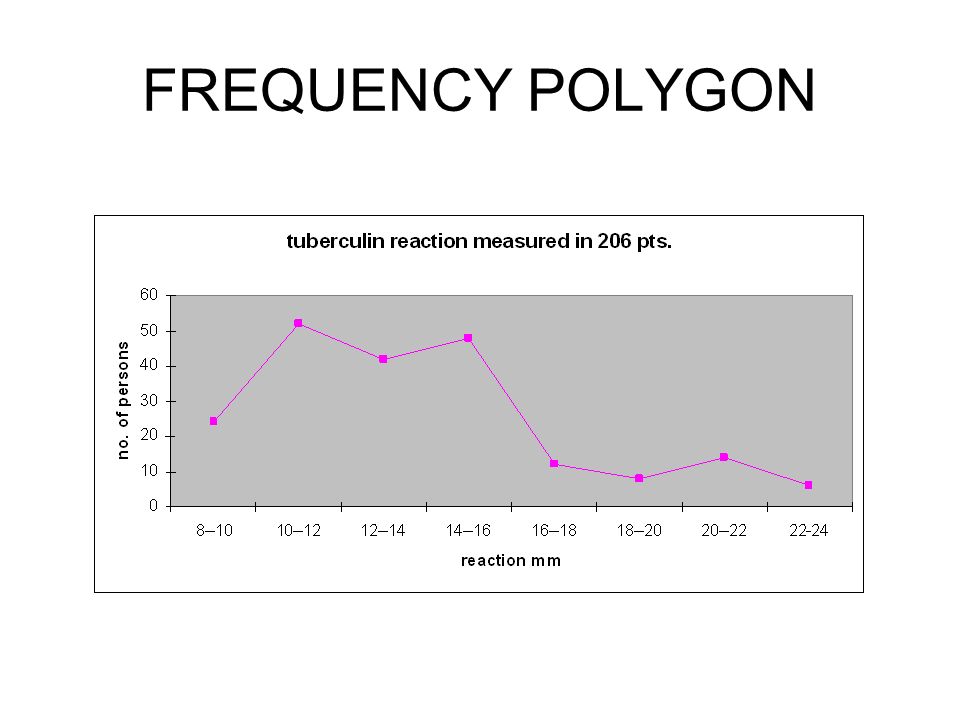
FREQUANCY DISTRIBUTION 8, 24, 18, 5, 6, 12, 4, 3, 3, 2, 3, 23, 9, 18, 16, 1, 2, 3, 5, 11, 13, 15, 9, 11, 11, 7, 10, 6, 5, 16, 20, 4, 3, 3, 3, 10, 3, 2, 1, 6, 9, 3, 7, 14, 8, 1, 4, 6, 4, 15, 22, 2, 1, 4, 7, 1, 12, 3, 23, 4, 19, 6, 2, 2, 4, 14, 2, 2, 21, 3, 2, 9, 3, 2, 1, 7, 19.

3
FREQUANCY DISTRIBUTION Age GroupFrequency 0-4IIII IIII IIII IIII IIII IIII IIII 35 5-9IIII IIII IIII III18 10-14IIII IIII I11 15-19IIII III8 20-24IIII I6

4
GRAPHIC AND DIAGRAMATIC PRESENTATION Useful method for presentation of data Impact on imagination of people Diagrams are better retained in mind of human. More attractive, Comparison of data

5
BAR CHART

6
COLUMN CHARTS

7
BAR CHART

8
MULTIPLE BAR CHART

9
COMPONENT BAR CHART

10
Frequency Polygon: It is obtained by joining mid points of the histogram blocks

11
FREQUENCY POLYGON

13
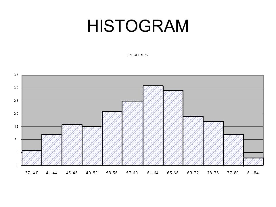
HISTOGRAM

14
Histogram Consists of adjacent rectangles having bases along x-axis and areas proportional to the class frequencies

15
HISTOGRAM

16
HISTORIGRAM It is a graph of time series Arrangement of data by their time of occurrence Time is marked on X-axis Variable is marked on Y-axis

17
HISTORIGRAM

18
LINEAR DIAGRAM

19
LINE DIAGRAM

20
HISTOGRAM

23
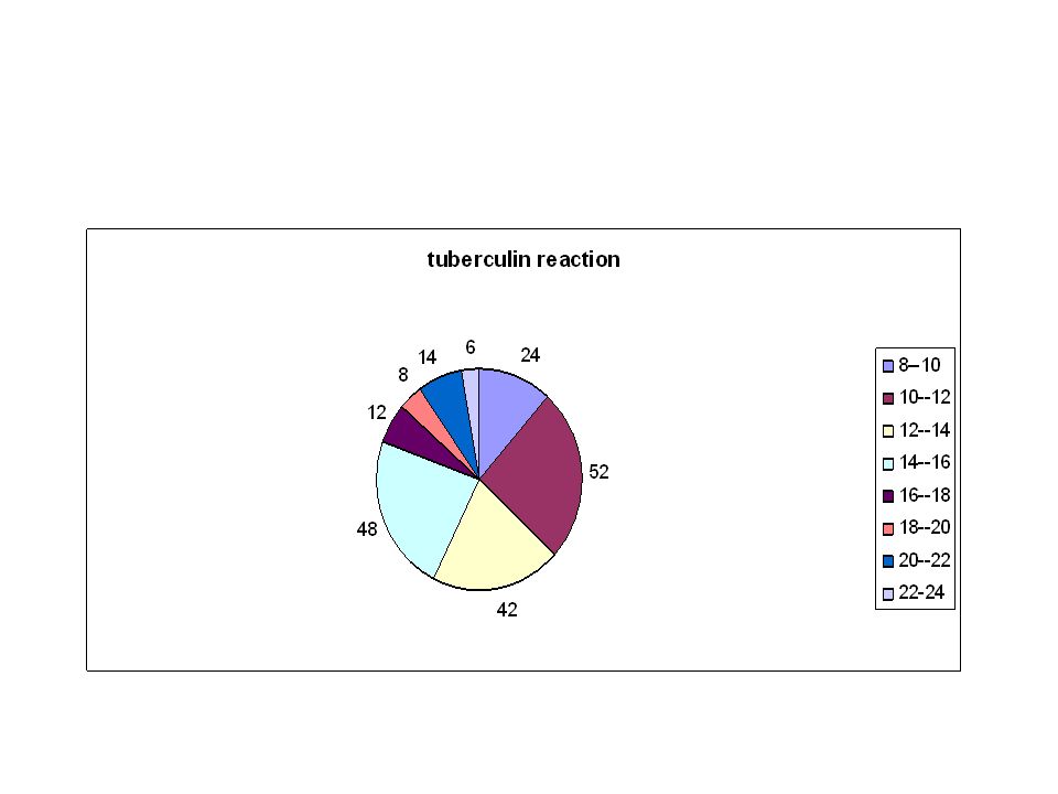
PIE CHART

25
RELATION B/W AGE AND WEIGHT

26
DIRECT RELATIONSHIP

27
SCATTER DIAGRAM

28
RELATIONSHIP OF AGE AND A DISEASE

29
ANALYSIS OF DATA When characteristic and frequency are both variable Calculation are: Averages Percentiles Standard deviation, Standard error Correlation and Regression coefficients.

30
NORMAL Normal is not the mean or a central value but the accepted range of variation on either side of mean or average. –Normal BP is not the mean but is a range between 100and 140 (mean 120 ± 20). Chances of even higher or lower are there.
. Chances of even higher or lower are there..")
31
HISTOGRAM

32
FREQUENCY CURVE When no. of observations is very large and group interval is reduced, the frequency polygon tends to lose its angulations giving place to a smooth curve known as frequency curve. This provides a continuous graph that is obtained in normal distribution of individuals in a large sample or of means in populations.

33
Normal distribution

34
Average We can find a single value which will represent all the values of the distribution in a definite way. The value used for this purpose to represent the distribution is called average. Averages tends to lie in the center of a distribution, they are called measures of central tendency.

35
It is difficult to learn anything by looking data which have not been properly arranged When data is arranged into a frequency distribution the information contained in the data understood. Features of data become clear when frequency distribution is represented by means of graph.

36
MEASURE OF CENTRAL TENDENCY “AVERAGE” What is the average or central value? How are the values dispersed around this value? Degree of scatter? Is the distribution normal ( shape of distribution)
.")
37
AVERAGE Average value of a characteristic is the one central value around which all other observations are dispersed. 50% of observations lie above and 50% of values lie below the central value. It helps To find most of normal observations lie close to central value Few of the too large or too small values lie far away at ends To find which group is better off by comparing the average of one group with that of other.

38
AVERAGE A term that describes the center of a series. Average or measure of central position –Mean –Median –Mode

39
Mean Most commonly used average. It is the value obtained by dividing the sum of the values by their number i.e., summarizing up of all observations and dividing total by no. of observations

40
MEAN It implies arithmetic average or arithmetic mean which is obtained by summing up all the observations and dividing by the total number of observations.e.g. ESRs of 7 patients are 7,5,4,6,4,5,9 Mean =7+5+4+6+4+5+9 =40/7=5.71 7

41
MEAN Tuberculin reaction of 10 boys was measured. find the mean? 5, 3, 8, 7, 8, 7, 9, 10, 11, 12 Mean=8mm

42
MEDIAN When all observations are arranged in either ascending or descending order, the middle observation is called as median. i.e. mid value of series. Median is a better indicator of central value when one or more of the lowest or highest observations are wide apart or not so evenly distributed.

43
MEDIAN 83, 75, 81, 79, 71, 95, 75, 77, 84, 79, 75, 71, 73, 91, 93. 71, 71, 73, 75, 75, 75, 77, 79, 79, 81, 83, 84, 91, 93, 95. Median = 79

44
MODE Most frequently occurring observation in a series I.e. the most common or most fashionable value. 85, 75, 81, 79, 71, 95, 75, 77, 75, 90, 71, 75, 79, 95, 75, 77, 84, 75, 81, 75.

45
MODE Most frequently occurring observation in a series I.e. the most common or most fashionable value. 85, 75, 81, 79, 71, 95, 75, 77, 75, 90, 71, 75, 79, 95, 75, 77, 84, 75, 81, 75. Mode = 75.

46
NORMAL DISTRIBUTION Normal curve Smooth, Bell shaped, bilaterally symmetrical curve Total area is =1 Mean is 0 Standard deviation=1 Mean, median, mode coincide. Area between X±1 SD=68.3% X±2SD=95.5% X±3SD=99.9%

47
Normal distribution

48
NORMAL DISTRIBUTION

49
POSITIVELY SKEWED

50
NEGATIVELY SKEWED

51
VARIABILITY Biological data are variable Two measurements in man are variable Cure rate are not equal but variable Height of students in same age group is not same but variable Height of students in one area is not same as compared to other place but variable Variability is essentially a normal character It is a biological phenomenon.

52
TYPES OF VARIABILITY Biological variability –That occurs within certain accepted biological limits. It occurs by chance. –Individual variability –Periodical variability –Class, group or category variability –Sampling variability or sampling error

53
REAL VARIABILITY –When the difference between two readings or observations or values of classes or samples is more than the defined limits in the universe, it is said to be real variability. The cause is external factors. e.g. significant difference in cure rates may be due to a better drug but not due to a chance.

54
Experimental variability Errors or differences due to materials, methods, procedures employed in the study or defects in the techniques involved in the experiment. –Observer error –Instrumental error –Sampling error.

Similar presentations