1. CS4402 – Parallel Computing
Lecture 5
Fox and Cannon Matrix Multiplication

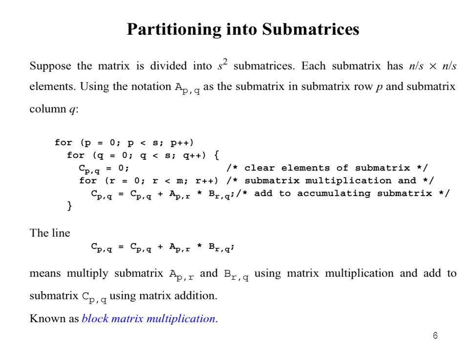
2. Matrix Multiplication
Start with two matrices A is n*m and B is m*p.
The product C=A*B is a matrix n*p.
The multiplication “row by column” gives a complexity of O(n*m*p).
Parallel Implementation  Linear Partitioning (I)
1.Scatter A to localA and Bcast B.
2. Compute localC = localA * B
3. Gather localC to C

3. Matrix Multiplication
Parallel Implementation  Linear Partitioning (II)
1. Bcast A and Scatter B on columns to localB.
2. Compute localC = A * localB
3. Gather the columns of localC to C
Advantages
1. Execution times reduce and the speedup increases.
2. Simple computation for each processor.
3. (Dis) for each element localC[i][j], the columns of B must be traversed.

4. Matrix Multiplication
Improvement of Parallel Implementation
1. Transpose the matrix B.
2. Scatter A to localA and Bcast B.
2. Compute the pseudo product localC = localA * B multiplying “row by row”
3. Gather localC to C
Memory cache overhead reduces.

5. Complexity of the Linear Multiplication
Scatter n*n/size elements:
Bcast n*n elements:
Compute the product:
Gather n*n/size elements:
Total Complexity: 5 5

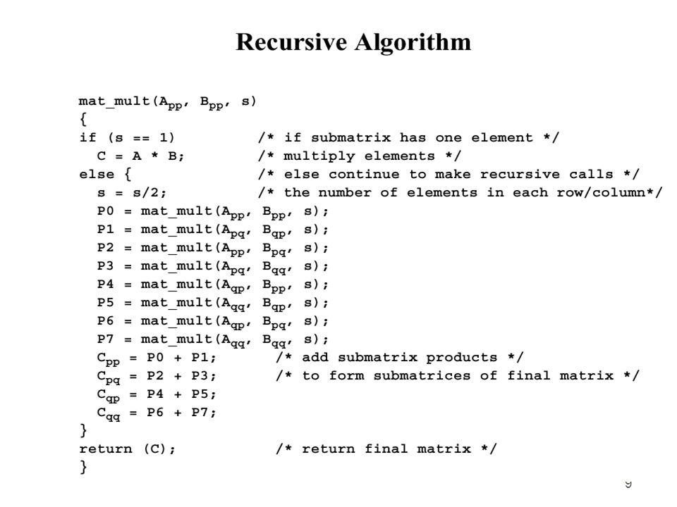
10. Strassen’s Algorithm

11. Fast Matrix Multiplication
Strassen: 7 multiplies, 18 additions, O(n2.81)
Strassen-Winograd: 7 multiplies, 15 additions
Coppersmith-Winograd, O(n2.376)
But this is not (easily) implementable
“Previous authors in this field have exhibited their algorithms directly, but we will have to rely on hashing and counting arguments to show the existence of a suitable algorithm.”

12. Grid Topology Grid Elements: - the dimension: 1, 2, 3 etc.
- the sizes of each dimension.
- the periodicity if the extreme are adjacent.
- reorder the processors.
MPI Methods:
- MPI_Cart_create() to create the grid.
- MPI_Card_coords() to get the coordinates
- MPI_Card_rank to find the rank.

13. MPI_Cart_create
Creates a communicator containing topology information.
int MPI_Cart_create(MPI_Comm comm_old, int ndims, int *dims, int *periods, int reorder, MPI_Comm *comm_cart);
MPI_Comm grid_comm;
int size[2], wrap_around[2], reorder;
size[0]=size[1]=q;
wrap_around[0]=1; wrap_around[1]=0;
reorder=1;
MPI_Cart_create(MPI_COMM_WORLD,2,size,wrap_around,reorder, &grid_comm);

14. MPI_Cart_coords, MPI_Cart_rank
MPI_Cart_coords(MPI_Comm comm,int rank,int maxdims,int *coords);
MPI_Cart_rank(MPI_Comm comm,int *coords,int *rank);
Find the coordinates/rank from rank/coordinates.
They map the ranks into coordinates.

15. How to find the rank of the neighbors
Consider that processor rank has got (row, col) as grid coordinate
1. Find the grid coordinates of the right/left neighbors and transform them into ranks.
leftCoords[0] = row; leftCoords[1]=(col-1)%size;
MPI_Cart_rank(grid, leftCoords, &leftRank);
2. void MPI_Cart_shift(MPI_Comm comm,int direction,int disp, int rank_source,int *rank_dest);
MPI_Cart_shift(grid, 1, -1, rank, &leftRank);

16. How to partition the matrix a
Some simple facts:
Processor 0 has the whole matrix so it needs to extract the blocks Ai,j
Processor 0 sends the block Ai,j to the processor of coords i,j.
Processor rank receives whatever Processor 0 sends.

17. How to partition + shift the matrix a
if(rank==0) for (i=0;i<p;i++)for(j=0;j<p;j++){
extract_matrix(n,n,a,n/p,n/p,local_a,i*n/p,j*n/p);
senderCoords[0]=i;senderCoords[1]=(j-i)%p;
MPI_Cart_rank(grid, senderCoords, &senderRank);
MPI_Send(&local_a[0][0], n*n/(p*p), MPI_INT, senderRank, tag1, MPI_COMM_WORLD); }
MPI_Recv(&local_a[0][0], n*n/(p*p), MPI_INT, 0, tag1, MPI_COMM_WORLD,&status_a);

19. Facts about the systolic computation
Consider the processor rank = (row, col).
- The processor rank computes for p-1 times
Receive a bloc from left in local_a.
Receive a block from above in local_b.
Compute the product local_a*local_b and accumulate it in local_c
Send local_a to right
Send local_b to below.
- The computation local_a*local_b takes place only after the processor’s receive is completed.
- Lots of processors are idle

20. C00 =A00 B00
A00
A10
A20
B00
B01
B02

21. C00 =A00 B00 +A01 B10
A01
A00
A10
A20
B10
B01
B02
B00

22. C00 =A00 B00 +A01 B10 +A02 B20 A02 A01 A00 A11 A10 A20 B20 B11 B02 B10

23. Some Other Facts
- The processing ends after 2*p-1 stages when processor (p-1, p-1) receives the last matrices.
- After p stages of processing some processors become idle. e.g. Processor (0,0)
- It remains the question of how we can reduce the number of stages to exact p-1.
Fox = Broadcast A, Multiply and roll B.
Cannon = Multiply, roll A, roll B.

24. Cannon’s Matrix Multiplication
- The matrix a is block partitioned as follows:
Row i of processors gets row i of blocks followed by shift << i positions.
A00
A01
A02
A10
A11
A12
A20
A21
A22
A00
A01
A02
A11
A12
A10
A22
A20
A21

25. Cannon’s Matrix Multiplication
- The matrix b is block partitioned on grid as follows:
Column i of processors gets column i of blocks followed by shifted up i positions.
B00
B01
B02
B10
B11
B12
B20
B21
B22
B00
B11
B22
B10
B21
B02
B20
B01
B12

26. Cannon’s Matrix Multiplication
For p times do the following computation
Multiply local_a with local_b.
Shift << local_a one position.
Shift up local_b one position.
A00
A01
A02
A11
A12
A10
A22
A20
A21
B00
B11
B22
B10
B21
B02
B20
B01
B12

27. C00 =A00 B00 Step 1. A00 A01 A02 A11 A12 A10 A22 A20 A21 B00 B11 B22

28. C00 =A00 B00 +A01 B10 Step 2. A01 A02 A00 A12 A10 A11 A20 A21 A22 B10

29. C00 =A00 B00 +A01 B10 +A02 B20 Step 3. A02 A00 A01 A10 A11 A12 A21 A22

30. Cannon Computation How to roll the matrices: Use send/receive
for(step=0;step<p;step++){
// calculate the product local a * local b and accumulate in local_c
cc = prod_matrix(n/p, n/p, n/p,local_a, local_b);
for(i=0;i<n/p;i++)for(j=0;j<n/p;j++) local_c[i][j] += cc[i][j];
// shift local a,
MPI_Send(&local_a[0][0], n*n/(p*p), MPI_INT, leftRank, tag1, MPI_COMM_WORLD);
MPI_Recv(&local_a[0][0], n*n/(p*p), MPI_INT, rightRank, tag1, MPI_COMM_WORLD,&status);
// shift b up
MPI_Send(&local_b[0][0], n*n/(p*p), MPI_INT, upRank, tag1, MPI_COMM_WORLD);
MPI_Recv(&local_b[0][0], n*n/(p*p), MPI_INT, downRank, tag1, MPI_COMM_WORLD,&status); }

31. Cannon Computation How to roll the matrices:
Use MPI_Send_recv_replace()
for(step=0;step<p;step++){
// calculate the product local a * local b and accumulate in local_c
cc = prod_matrix(n/p, n/p, n/p,local_a, local_b);
for(i=0;i<n/p;i++)for(j=0;j<n/p;j++) local_c[i][j] += cc[i][j];
// shift local a, local_b
MPI_Send_recv_replace(&local_a[0][0], n*n/(p*p), MPI_INT, leftRank, tag1, rightRank,
tag2, MPI_COMM_WORLD, &status);
MPI_Send_recv_replace (&local_b[0][0], n*n/(p*p), MPI_INT, upRank, tag1, downRank, }

32. Cannon’s Complexity
Evaluate the complexity in terms of n and p = sqrt(size).
The matrices a and b are sent to the grid with one send operation 
Each processor computes p matrix multiplications in 
Each processor does p rolls of local_a and local_b 
- Total execution time is 

33. Simple Comparisons: Complexities: Cannon: Linear:
Each strategy uses same amount of computation.
Cannon uses less communication.
Cannon uses smaller matrices. 33 33

34. Fox’s Matrix Multiplication (1)
- The row i of blocks is broadcasted to the row i of processors in the order Ai,i Ai,i+1 Ai,i+2 …Ai,i-1
- The matrix b is partitioned on grid row after row in the normal order.
- In this way each processor has a block of A and a block of B and it can proceed to computation.
- After computation roll the matrix b up

35. Fox’s Matrix Multiplication (2)
Consider the processor rank = (row, col).
Step 1. Partition the matrix b on the grid so that Bi,j goes to Pi,j.
Step 2. For i=0,1,2,..,p-1 times do
Broadcast Arow, row+i to all the processors of the same row.
Multiply local_a by local_b and accumulate the product to local_c
Send local_b to (row-1, col)
Receive in local_b from (row+1, col)

36. Step 1.
C00 =A00 B00
A00
A11
A22
B00
B01
B02
B10
B11
B12
B20
B21
B22

37. C00 =A00 B00 +A01 B10 Step 2. A01 A12 A20 B10 B11 B12 B20 B21 B22 B00

38. C00 =A00 B00 +A01 B10 +A02 B20 Step 3. A02 A10 A21 B20 B21 B22 B00 B01