1. 1/68: Topic 1.3 – Linear Panel Data Regression Microeconometric Modeling William Greene Stern School of Business New York University New York NY USA William Greene Stern School of Business New York University New York NY USA 1.3 Linear Panel Data Regression Models

2. 2/68: Topic 1.3 – Linear Panel Data Regression Concepts Unbalanced Panel Cluster Estimator Block Bootstrap Difference in Differences Incidental Parameters Problem Endogeneity Instrumental Variable Control Function Estimator Mundlak Form Correlated Random Effects Hausman Test Lagrange Multiplier (LM) Test Variable Addition (Wu) Test Models Linear Regression Fixed Effects LR Model Random Effects LR Model

3. 3/68: Topic 1.3 – Linear Panel Data Regression

4. 4/68: Topic 1.3 – Linear Panel Data Regression

5. 5/68: Topic 1.3 – Linear Panel Data Regression

6. 6/68: Topic 1.3 – Linear Panel Data Regression BHPS Has Evolved

7. 7/68: Topic 1.3 – Linear Panel Data Regression German Socioeconomic Panel

8. 8/68: Topic 1.3 – Linear Panel Data Regression Balanced and Unbalanced Panels  Distinction: Balanced vs. Unbalanced Panels  A notation to help with mechanics z i,t, i = 1,…,N; t = 1,…,T i  The role of the assumption Mathematical and notational convenience:  Balanced, n=NT  Unbalanced: The fixed T i assumption almost never necessary. If unbalancedness is due to nonrandom attrition from an otherwise balanced panel, then this will require special considerations.

9. 9/68: Topic 1.3 – Linear Panel Data Regression An Unbalanced Panel: RWM’s GSOEP Data on Health Care N = 7,293 Households Some households exited then returned

10. 10/68: Topic 1.3 – Linear Panel Data Regression Cornwell and Rupert Data Cornwell and Rupert Returns to Schooling Data, 595 Individuals, 7 Years (Extracted from NLSY.) Variables in the file are EXP = work experience WKS = weeks worked OCC = occupation, 1 if blue collar, IND = 1 if manufacturing industry SOUTH = 1 if resides in south SMSA= 1 if resides in a city (SMSA) MS = 1 if married FEM = 1 if female UNION = 1 if wage set by union contract ED = years of education LWAGE = log of wage = dependent variable in regressions These data were analyzed in Cornwell, C. and Rupert, P., "Efficient Estimation with Panel Data: An Empirical Comparison of Instrumental Variable Estimators," Journal of Applied Econometrics, 3, 1988, pp. 149-155. See Baltagi, page 122 for further analysis. The data were downloaded from the website for Baltagi's text.

11. 11/68: Topic 1.3 – Linear Panel Data Regression

12. 12/68: Topic 1.3 – Linear Panel Data Regression Common Effects Models  Unobserved individual effects in regression: E[y it | x it, c i ] Notation:  Linear specification: Fixed Effects: E[c i | X i ] = g(X i ). Cov[x it,c i ] ≠0 effects are correlated with included variables. Random Effects: E[c i | X i ] = μ; effects are uncorrelated with included variables. If X i contains a constant term, μ=0 WLOG. Common: Cov[x it,c i ] =0, but E[c i | X i ] = μ is needed for the full model

13. 13/68: Topic 1.3 – Linear Panel Data Regression Convenient Notation  Fixed Effects – the ‘dummy variable model’  Random Effects – the ‘error components model’ Individual specific constant terms. Compound (“composed”) disturbance

14. 14/68: Topic 1.3 – Linear Panel Data Regression Estimating β  β is the partial effect of interest  Can it be estimated (consistently) in the presence of (unmeasured) c i ? Does pooled least squares “work?” Strategies for “controlling for c i ” using the sample data.

15. 15/68: Topic 1.3 – Linear Panel Data Regression 1. The Pooled Regression  Presence of omitted effects  Potential bias/inconsistency of OLS – Depends on ‘fixed’ or ‘random’ If FE, X is endogenous: Omitted Variables Bias If RE, OLS is OK but standard errors are incorrect.

16. 16/68: Topic 1.3 – Linear Panel Data Regression OLS with Individual Effects The omitted variable(s) are the group means

17. 17/68: Topic 1.3 – Linear Panel Data Regression Ordinary Least Squares  Standard results for OLS in a generalized regression model Consistent if RE, inconsistent if FE. Unbiased for something in either case. Inefficient in all cases.  True Variance

18. 18/68: Topic 1.3 – Linear Panel Data Regression Estimating the Sampling Variance of b  b may or may not be consistent for . We estimate its variance regardless  s 2 (X X) -1 is not the correct matrix Correlation across observations: Yes Heteroscedasticity: Maybe  Is there a “robust” covariance matrix? Robust estimation (in general) The White estimator for heteroscedasticity A Robust estimator for OLS.

19. 19/68: Topic 1.3 – Linear Panel Data Regression A Cluster Estimator

20. 20/68: Topic 1.3 – Linear Panel Data Regression Alternative OLS Variance Estimators Cluster correction increases SEs +---------+--------------+----------------+--------+---------+ |Variable | Coefficient | Standard Error |b/St.Er.|P[|Z|>z] | +---------+--------------+----------------+--------+---------+ Constant 5.40159723.04838934 111.628.0000 EXP.04084968.00218534 18.693.0000 EXPSQ -.00068788.480428D-04 -14.318.0000 OCC -.13830480.01480107 -9.344.0000 SMSA.14856267.01206772 12.311.0000 MS.06798358.02074599 3.277.0010 FEM -.40020215.02526118 -15.843.0000 UNION.09409925.01253203 7.509.0000 ED.05812166.00260039 22.351.0000 Robust Constant 5.40159723.10156038 53.186.0000 EXP.04084968.00432272 9.450.0000 EXPSQ -.00068788.983981D-04 -6.991.0000 OCC -.13830480.02772631 -4.988.0000 SMSA.14856267.02423668 6.130.0000 MS.06798358.04382220 1.551.1208 FEM -.40020215.04961926 -8.065.0000 UNION.09409925.02422669 3.884.0001 ED.05812166.00555697 10.459.0000

21. 21/68: Topic 1.3 – Linear Panel Data Regression Results of Bootstrap Estimation

22. 22/68: Topic 1.3 – Linear Panel Data Regression Bootstrap variance for a panel data estimator  Panel Bootstrap = Block Bootstrap  Data set is N groups of size T i  Bootstrap sample is N groups of size T i drawn with replacement. The bootstrap replication must account for panel data nature of the data set.

23. 23/68: Topic 1.3 – Linear Panel Data Regression

24. 24/68: Topic 1.3 – Linear Panel Data Regression Difference-in-Differences Model With two periods and strict exogeneity of D and T, This is a linear regression model. If there are no regressors,

25. 25/68: Topic 1.3 – Linear Panel Data Regression Difference in Differences

26. 26/68: Topic 1.3 – Linear Panel Data Regression UK Office of Fair Trading, May 2012; Stephen Davies http://dera.ioe.ac.uk/14610/1/oft1416.pdf

27. 27/68: Topic 1.3 – Linear Panel Data Regression Outcome is the fees charged. Activity is collusion on fees.

28. 28/68: Topic 1.3 – Linear Panel Data Regression Treatment Schools: Treatment is an intervention by the Office of Fair Trading Control Schools were not involved in the conspiracy Treatment is not voluntary

29. 29/68: Topic 1.3 – Linear Panel Data Regression Apparent Impact of the Intervention

30. 30/68: Topic 1.3 – Linear Panel Data Regression

31. 31/68: Topic 1.3 – Linear Panel Data Regression Treatment (Intervention) Effect =  1 +  2 if SS school

32. 32/68: Topic 1.3 – Linear Panel Data Regression In order to test robustness two versions of the fixed effects model were run. The first is Ordinary Least Squares, and the second is heteroscedasticity and auto-correlation robust (HAC) standard errors in order to check for heteroscedasticity and autocorrelation.

33. 33/68: Topic 1.3 – Linear Panel Data Regression

34. 34/68: Topic 1.3 – Linear Panel Data Regression The cumulative impact of the intervention is the area between the two paths from intervention to time T.

35. 35/68: Topic 1.3 – Linear Panel Data Regression

36. 36/68: Topic 1.3 – Linear Panel Data Regression 2. Estimation with Fixed Effects  The fixed effects model  c i is arbitrarily correlated with x it but E[ε it |X i,c i ]=0  Dummy variable representation

37. 37/68: Topic 1.3 – Linear Panel Data Regression The Fixed Effects Model y i = X i  + d i  i + ε i, for each individual E[c i | X i ] = g(X i ); Effects are correlated with included variables. Cov[x it,c i ] ≠0

38. 38/68: Topic 1.3 – Linear Panel Data Regression Estimating the Fixed Effects Model  The FEM is a plain vanilla regression model but with many independent variables  Least squares is unbiased, consistent, efficient, but inconvenient if N is large.

39. 39/68: Topic 1.3 – Linear Panel Data Regression The Within Transformation Removes the Effects Wooldridge notation for data in deviations from group means

40. 40/68: Topic 1.3 – Linear Panel Data Regression Least Squares Dummy Variable Estimator  b is obtained by ‘within’ groups least squares (group mean deviations)  Normal equations for a are D’Xb+D’Da=D’y a = (D’D) -1 D’(y – Xb) Notes: This is simple algebra – the estimator is just OLS Least squares is an estimator, not a model. (Repeat twice.) Note what a i is when T i = 1. Follow this with y it -a i -x it ’b=0 if T i =1.

41. 41/68: Topic 1.3 – Linear Panel Data Regression Inference About OLS  Assume strict exogeneity: Cov[ε it,(x js,c j )]=0. Every disturbance in every period for each person is uncorrelated with variables and effects for every person and across periods.  Now, it’s just least squares in a classical linear regression model.  Asy.Var[b] =

42. 42/68: Topic 1.3 – Linear Panel Data Regression Application Cornwell and Rupert

43. 43/68: Topic 1.3 – Linear Panel Data Regression LSDV Results Pooled OLS Note huge changes in the coefficients. SMSA and MS change signs. Significance changes completely.

44. 44/68: Topic 1.3 – Linear Panel Data Regression Estimated Fixed Effects

45. 45/68: Topic 1.3 – Linear Panel Data Regression The Effect of the Effects R 2 rises from.26510 to.90542

46. 46/68: Topic 1.3 – Linear Panel Data Regression Robust Covariance Matrix for LSDV Cluster Estimator for Within Estimator Effect is less pronounced than for OLS

47. 47/68: Topic 1.3 – Linear Panel Data Regression Endogeneity in the FEM y i = X i  + d i α i + ε i for each individual E[w i | X i ] = g(X i ); Effects are correlated with included variables. Cov[x it,w i ] ≠0 X is endogenous because of the correlation between x it and w i

48. 48/68: Topic 1.3 – Linear Panel Data Regression The within (LSDV) estimator is an instrumental variable (IV) estimator

49. 49/68: Topic 1.3 – Linear Panel Data Regression LSDV is a Control Function Estimator

50. 50/68: Topic 1.3 – Linear Panel Data Regression LSDV is a Control Function Estimator

51. 51/68: Topic 1.3 – Linear Panel Data Regression The problem here is the estimator of the disturbance variance. The matrix is OK. Note, for example,.01374007/.01950085 (top panel) =.16510 /.23432 (bottom panel).

52. 52/68: Topic 1.3 – Linear Panel Data Regression

53. 53/68: Topic 1.3 – Linear Panel Data Regression 3. The Random Effects Model The random effects model c i is uncorrelated with x it for all t; E[c i |X i ] = 0 E[ε it |X i,c i ]=0

54. 54/68: Topic 1.3 – Linear Panel Data Regression Random vs. Fixed Effects  Random Effects Small number of parameters Efficient estimation Objectionable orthogonality assumption (c i  X i )  Fixed Effects Robust – generally consistent Large number of parameters More reasonable assumption Precludes time invariant regressors   Which is the more reasonable model?

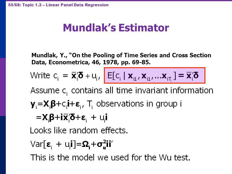
55. 55/68: Topic 1.3 – Linear Panel Data Regression Mundlak’s Estimator Mundlak, Y., “On the Pooling of Time Series and Cross Section Data, Econometrica, 46, 1978, pp. 69-85.

56. 56/68: Topic 1.3 – Linear Panel Data Regression Mundlak Form of FE Model +--------+--------------+----------------+--------+--------+----------+ |Variable| Coefficient | Standard Error |b/St.Er.|P[|Z|>z]| Mean of X| +--------+--------------+----------------+--------+--------+----------+ x(i,t) OCC | -.02021384.01375165 -1.470.1416.51116447 SMSA | -.04250645.01951727 -2.178.0294.65378151 MS | -.02946444.01915264 -1.538.1240.81440576 EXP |.09665711.00119262 81.046.0000 19.8537815 z(i) FEM | -.34322129.05725632 -5.994.0000.11260504 ED |.05099781.00575551 8.861.0000 12.8453782 Means of x(I,t) and constant Constant| 5.72655261.10300460 55.595.0000 OCCB | -.10850252.03635921 -2.984.0028.51116447 SMSAB |.22934020.03282197 6.987.0000.65378151 MSB |.20453332.05329948 3.837.0001.81440576 EXPB | -.08988632.00165025 -54.468.0000 19.8537815 Estimates: Var[e] =.0235632 Var[u] =.0773825

57. 57/68: Topic 1.3 – Linear Panel Data Regression A “Hierarchical” Model

58. 58/68: Topic 1.3 – Linear Panel Data Regression Mundlak’s Approach for an FE Model with Time Invariant Variables

59. 59/68: Topic 1.3 – Linear Panel Data Regression Correlated Random Effects

60. 60/68: Topic 1.3 – Linear Panel Data Regression LM Tests +--------------------------------------------------+ | Random Effects Model: v(i,t) = e(i,t) + u(i) | Unbalanced Panel | Estimates: Var[e] =.216794D+02 | #(T=1) = 1525 | Var[u] =.958560D+01 | #(T=2) = 1079 | Corr[v(i,t),v(i,s)] =.306592 | #(T=3) = 825 | Lagrange Multiplier Test vs. Model (3) = 4419.33 | #(T=4) = 926 | ( 1 df, prob value =.000000) | #(T=5) = 1051 | (High values of LM favor FEM/REM over CR model.) | #(T=6) = 1200 | Baltagi-Li form of LM Statistic = 1618.75 | #(T=7) = 887 +--------------------------------------------------+ | Random Effects Model: v(i,t) = e(i,t) + u(i) | | Estimates: Var[e] =.210257D+02 | Balanced Panel | Var[u] =.860646D+01 | T = 7 | Corr[v(i,t),v(i,s)] =.290444 | | Lagrange Multiplier Test vs. Model (3) = 1561.57 | | ( 1 df, prob value =.000000) | | (High values of LM favor FEM/REM over CR model.) | | Baltagi-Li form of LM Statistic = 1561.57 | +--------------------------------------------------+ REGRESS ; Lhs=docvis ; Rhs=one,hhninc,age,female,educ ; panel $

61. 61/68: Topic 1.3 – Linear Panel Data Regression A One Way REM

62. 62/68: Topic 1.3 – Linear Panel Data Regression A Hausman Test for FE vs. RE EstimatorRandom Effects E[c i |X i ] = 0 Fixed Effects E[c i |X i ] ≠ 0 FGLS (Random Effects) Consistent and Efficient Inconsistent LSDV (Fixed Effects) Consistent Inefficient Consistent Possibly Efficient

63. 63/68: Topic 1.3 – Linear Panel Data Regression Hausman Test for Effects

64. 64/68: Topic 1.3 – Linear Panel Data Regression Hausman There is a built in procedure for this. It is not always appropriate to compare estimators this way.

65. 65/68: Topic 1.3 – Linear Panel Data Regression A Variable Addition Test  Asymptotically equivalent to Hausman  Also equivalent to Mundlak formulation  In the random effects model, using FGLS Only applies to time varying variables Add expanded group means to the regression (i.e., observation i,t gets same group means for all t. Use standard F or Wald test to test for coefficients on means equal to 0. Large F or chi-squared weighs against random effects specification.

66. 66/68: Topic 1.3 – Linear Panel Data Regression Variable Addition

67. 67/68: Topic 1.3 – Linear Panel Data Regression Application: Wu Test NAMELIST ; XV = exp,expsq,wks,occ,ind,south,smsa,ms,union$ NAMELIST ; (new) xmeans = expb,expsqb,wksb,occb,indb,southb,smsab,msb,unionb $ CREATE ; xmeans = Group Mean(xv,pds=ti) $ REGRESS ; Lhs = lwage ; Rhs = xmeans,Xv,ed,fem,one ; panel ; random ; Test: xmeans $

68. 68/68: Topic 1.3 – Linear Panel Data Regression Means Added