1. Peripheral drift illusion

3. Multiple views Hartley and Zisserman Lowe stereo vision structure from motion optical flow

4. Why multiple views? Structure and depth are inherently ambiguous from single views. Images from Lana Lazebnik

5. Why multiple views? Structure and depth are inherently ambiguous from single views. Optical center P1 P2 P1’=P2’

6. Camera parameters Camera frame 1 Intrinsic parameters: Image coordinates relative to camera  Pixel coordinates Extrinsic parameters: Camera frame 1  Camera frame 2 Camera frame 2 Extrinsic params: rotation matrix and translation vector Intrinsic params: focal length, pixel sizes (mm), image center point, radial distortion parameters We’ll assume for now that these parameters are given and fixed.

7. Geometry for a simple stereo system First, assuming parallel optical axes, known camera parameters (i.e., calibrated cameras):

8. baseline optical center (left) optical center (right) Focal length World point image point (left) image point (right) Depth of p

9. Assume parallel optical axes, known camera parameters (i.e., calibrated cameras). What is expression for Z? Similar triangles (p l, P, p r ) and (O l, P, O r ): Geometry for a simple stereo system disparity

10. Depth from disparity image I(x,y) image I´(x´,y´) Disparity map D(x,y) (x´,y´)=(x+D(x,y), y) So if we could find the corresponding points in two images, we could estimate relative depth…

11. What did we need to know? Correspondence for every pixel. Sort of like project 2, but project 2 is “sparse” and we need “dense” correspondence. Calibration for the cameras.

12. Where do we need to search?

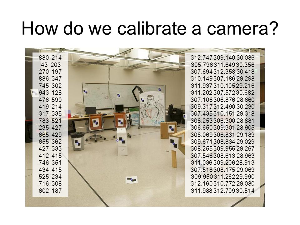
13. How do we calibrate a camera? 312.747 309.140 30.086 305.796 311.649 30.356 307.694 312.358 30.418 310.149 307.186 29.298 311.937 310.105 29.216 311.202 307.572 30.682 307.106 306.876 28.660 309.317 312.490 30.230 307.435 310.151 29.318 308.253 306.300 28.881 306.650 309.301 28.905 308.069 306.831 29.189 309.671 308.834 29.029 308.255 309.955 29.267 307.546 308.613 28.963 311.036 309.206 28.913 307.518 308.175 29.069 309.950 311.262 29.990 312.160 310.772 29.080 311.988 312.709 30.514 880 214 43 203 270 197 886 347 745 302 943 128 476 590 419 214 317 335 783 521 235 427 665 429 655 362 427 333 412 415 746 351 434 415 525 234 716 308 602 187

14. World vs Camera coordinates

15. Image formation Let’s design a camera – Idea 1: put a piece of film in front of an object – Do we get a reasonable image? Slide source: Seitz

16. Pinhole camera Idea 2: add a barrier to block off most of the rays – This reduces blurring – The opening known as the aperture Slide source: Seitz

17. Pinhole camera Figure from Forsyth f f = focal length c = center of the camera c

18. Projection: world coordinates  image coordinates X

19. Homogeneous coordinates Conversion Converting to homogeneous coordinates homogeneous image coordinates homogeneous scene coordinates Converting from homogeneous coordinates

20. World vs Camera coordinates

21. Slide Credit: Saverese Projection matrix x: Image Coordinates: (u,v,1) K: Intrinsic Matrix (3x3) R: Rotation (3x3) t: Translation (3x1) X: World Coordinates: (X,Y,Z,1) OwOw iwiw kwkw jwjw R,T

22. Pinhole Camera Model x: Image Coordinates: (u,v,1) K: Intrinsic Matrix (3x3) R: Rotation (3x3) t: Translation (3x1) X: World Coordinates: (X,Y,Z,1)

23. K Slide Credit: Saverese Projection matrix Intrinsic Assumptions Unit aspect ratio Optical center at (0,0) No skew Extrinsic Assumptions No rotation Camera at (0,0,0)

24. Remove assumption: known optical center Intrinsic Assumptions Unit aspect ratio No skew Extrinsic Assumptions No rotation Camera at (0,0,0)

25. Remove assumption: square pixels Intrinsic Assumptions No skew Extrinsic Assumptions No rotation Camera at (0,0,0)

26. Remove assumption: non-skewed pixels Intrinsic AssumptionsExtrinsic Assumptions No rotation Camera at (0,0,0) Note: different books use different notation for parameters

27. Oriented and Translated Camera OwOw iwiw kwkw jwjw t R

28. Allow camera translation Intrinsic AssumptionsExtrinsic Assumptions No rotation

29. 3D Rotation of Points, : Rotation around the coordinate axes, counter-clockwise: p p’p’p’p’  y z Slide Credit: Saverese

30. Allow camera rotation

31. Degrees of freedom 56

32. Beyond Pinholes: Radial Distortion Common in wide-angle lenses or for special applications (e.g., security) Creates non-linear terms in projection Usually handled by through solving for non-linear terms and then correcting image Image from Martin Habbecke Corrected Barrel Distortion

33. How to calibrate the camera?

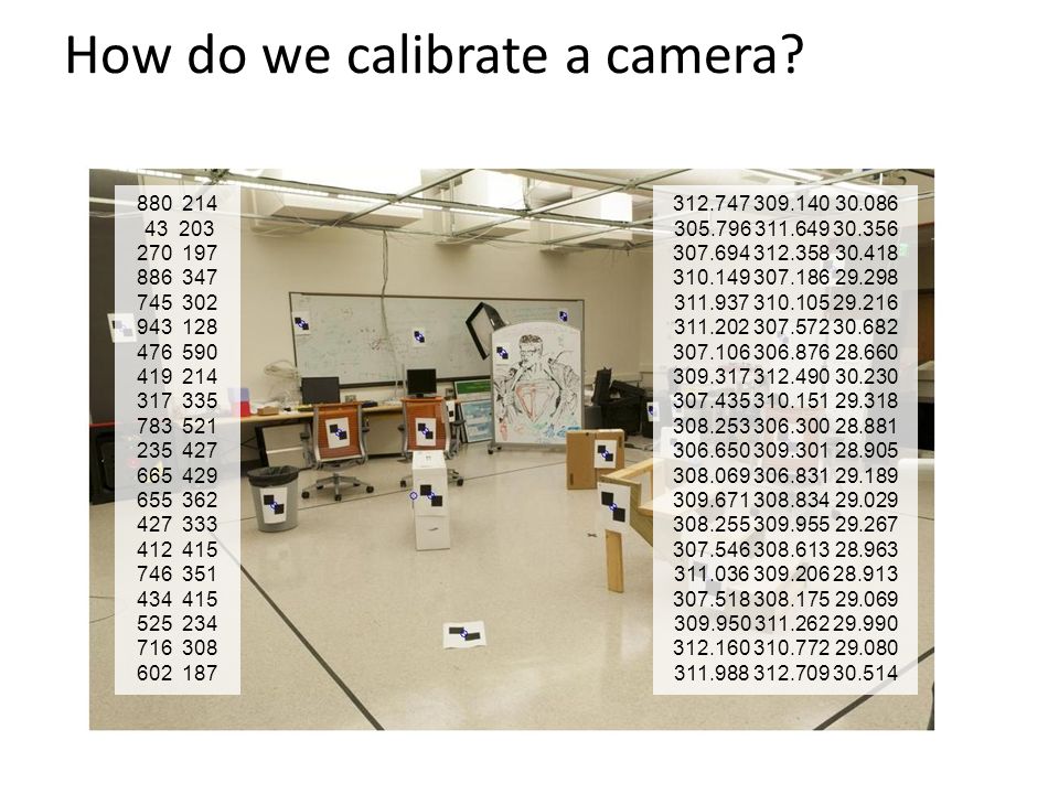
34. Calibrating the Camera Use an scene with known geometry – Correspond image points to 3d points – Get least squares solution (or non-linear solution)

35. How do we calibrate a camera? 312.747 309.140 30.086 305.796 311.649 30.356 307.694 312.358 30.418 310.149 307.186 29.298 311.937 310.105 29.216 311.202 307.572 30.682 307.106 306.876 28.660 309.317 312.490 30.230 307.435 310.151 29.318 308.253 306.300 28.881 306.650 309.301 28.905 308.069 306.831 29.189 309.671 308.834 29.029 308.255 309.955 29.267 307.546 308.613 28.963 311.036 309.206 28.913 307.518 308.175 29.069 309.950 311.262 29.990 312.160 310.772 29.080 311.988 312.709 30.514 880 214 43 203 270 197 886 347 745 302 943 128 476 590 419 214 317 335 783 521 235 427 665 429 655 362 427 333 412 415 746 351 434 415 525 234 716 308 602 187

36. Method 1 – homogeneous linear system Solve for m’s entries using linear least squares Ax=0 form [U, S, V] = svd(A); M = V(:,end); M = reshape(M,[],3)';

37. Method 2 – nonhomogeneous linear system Solve for m’s entries using linear least squares Ax=b form M = A\Y; M = [M;1]; M = reshape(M,[],3)';

38. Calibration with linear method Advantages – Easy to formulate and solve – Provides initialization for non-linear methods Disadvantages – Doesn’t directly give you camera parameters – Doesn’t model radial distortion – Can’t impose constraints, such as known focal length Non-linear methods are preferred – Define error as difference between projected points and measured points – Minimize error using Newton’s method or other non-linear optimization