1. tom.h.wilson wilson@geo.wvu.edu Department of Geology and Geography West Virginia University Morgantown, WV

2. Autocorrelation involves simple calculations repeated for each lag or shift Shift -Multiply - Sum

3. 0-lag autocorrelation = 1 Notice that at this lag the two series are 180 degrees out of phase and we get a negative correlation The following two lags (B and C) yield positive correlation

4. Autocorrelation of a sine wave with itself.

5. Truly random variations of observations through time or space will have nearly zero autocorrelation at all lags except for the 0- lag.

6. Autocorrelation helps eliminate noise, but it cannot do this entirely. The autocorrelation of this noisy signal reveals an imbedded periodic component, but the argument for its presence (basically an interpretation) may be perceived as weak.

7. The appearance of the autocorrelation of a series of numbers (your data measured at regular intervals) will be influenced by the presence of long term (or wavelength)rising or falling trends.

8. Imbedded “signal” - a simple sine wave. The variations we are searching for. “Noise” The noise could be attributed to other random factor that produce variability on the quantity being measured or to measurement error itself. Long period (or wavelength ) rise in value superimposed on the short period (short wavelength) variations in the “signal” A summation of the sine wave plus noise Summation of sine wave, noise, and long term rise in value. Autocorrelation of series shown at left

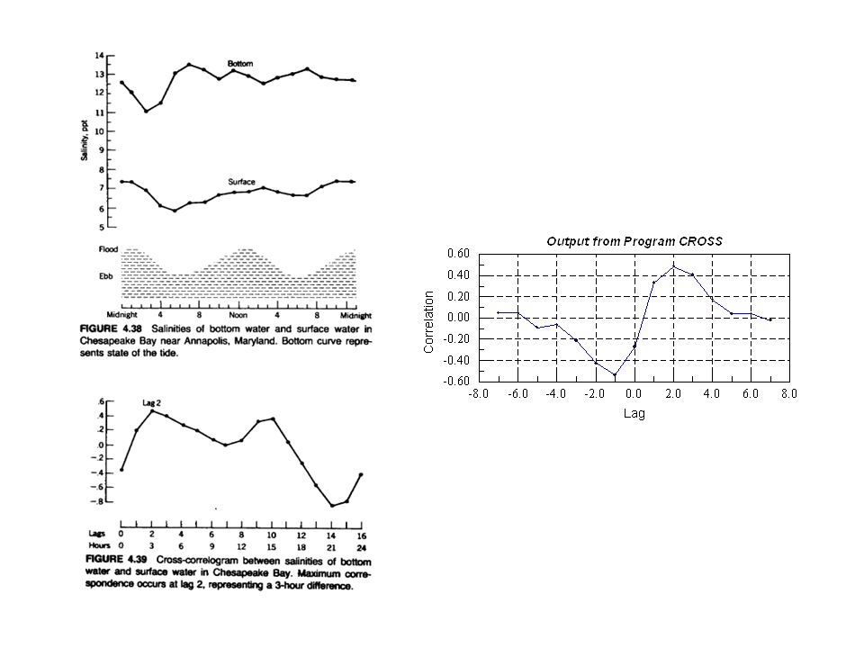
9. The autocorrelation is symmetrical The cross correlation is asymmetrical.

13. File that is entered first is shifted to the left relative to the second input file to obtain the positive lag.

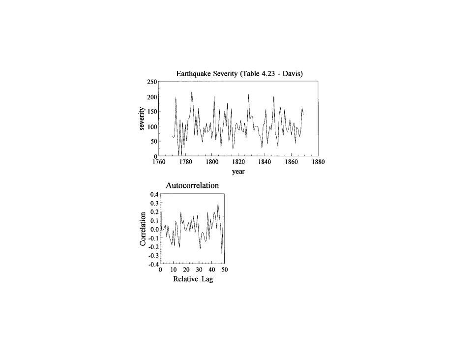
14. It’s difficult to make arguments for definitive peaks in this autocorrelation, however, in today’s lab exercise you’ll have the opportunity to investigate this further by looking at the cross correlation between Del O in the Mediterranean and Caribbean seas.

15. Again, recall the effect of random noise on the autocorrelation and crosscorrrelation.

16. Remember, the autocorrelation helps eliminate noise, but it cannot do this entirely. The autocorrelation of noisy signal such as the one at left may hint at the presence of imbedded periodic components, but the argument for their presence (basically an interpretation) may be perceived as weak.

17. Begin working on the lab assignment, and for today, hand in a plot of the autocorrelation the  18 O measurements from the Caribbean sea. (Due at the end of today’s class) Interpret the autocorrelation and mark peaks and/or troughs you feel suggest the presence of periodic variation within the  18 O variations. Label your plot and specifically note the period(s) marked off by features in the autocorrelation.