1. Multivariate Data Summary

2. Linear Regression and Correlation

3. Pearson’s correlation coefficient r.

4. Slope and Intercept of the Least Squares line

5. Scatter Plot Patterns r = 0.0 r = +0.7 r = +0.9r = +1.0

6. r = -0.7 r = -0.9r = -1.0

7. Non-Linear Patterns r can take on arbitrary values between -1 and +1 if the pattern is non-linear depending or how well your can fit a straight line to the pattern

8. The Coefficient of Determination

9. An important Identity in Statistics (Total variability in Y) = (variability in Y explained by X) + (variability in Y unexplained by X)

10. It can also be shown: = proportion variability in Y explained by X. = the coefficient of determination

11. Categorical Data Techniques for summarizing, displaying and graphing

12. The frequency table The bar graph Suppose we have collected data on a categorical variable X having k categories – 1, 2, …, k. To construct the frequency table we simply count for each category (i) of X, the number of cases falling in that category (f i ) To plot the bar graph we simply draw a bar of height f i above each category (i) of X.

13. Example In this example data has been collected for n = 34,188 subjects. The purpose of the study was to determine the relationship between the use of Antidepressants, Mood medication, Anxiety medication, Stimulants and Sleeping pills. In addition the study interested in examining the effects of the independent variables (gender, age, income, education and role) on both individual use of the medications and the multiple use of the medications.

14. The variables were: 1.Antidepressant use, 2.Mood medication use, 3.Anxiety medication use, 4.Stimulant use and 5.Sleeping pills use. 6.gender, 7.age, 8.income, 9.education and 10.Role – i.Parent, worker, partner ii.Parent, partner iii.Parent, worker iv.worker, partner v.worker only vi.Parent only vii.Partner only viii.No roles

15. Frequency Table for Age

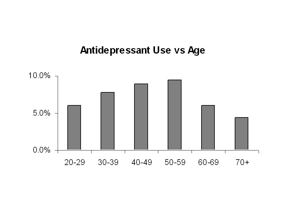
16. Bar Graph for Age

17. Frequency Table for Role

18. Bar Graph for Role

19. The pie chart An alternative to the bar chart Draw a circle (a pie) Divide the circle into segments with area of each segment proportional to f i or p i = f i /n

20. Example In this study the population are individuals who received a head injury. (n = 22540) The variable is the mechanism that caused the head injury (InjMech) with categories: –MVA (Motor vehicle accident) –Falls –Violence –Other VA (Other vehicle accidents) –Accidents (industrial accident) –Other (all other mechanisms for head injury)

21. Graphical and Tabular Display of Categorical Data. The frequency table The bar graph The pie chart

22. The frequency table

23. The bar graph

24. The pie chart

25. Multivariate Categorical Data

26. The two way frequency table The  2 statistic Techniques for examining dependence amongst two categorical variables

27. Situation We have two categorical variables R and C. The number of categories of R is r. The number of categories of C is c. We observe n subjects from the population and count x ij = the number of subjects for which R = i and C = j. R = rows, C = columns

28. Example Both Systolic Blood pressure (C) and Serum Chlosterol (R) were meansured for a sample of n = 1237 subjects. The categories for Blood Pressure are: <126127-146147-166167+ The categories for Chlosterol are: <200200-219220-259260+

29. Table: two-way frequency Serum Cholesterol Systolic Blood pressure <127127-146147-166167+ Total < 200 1171214722307 200-219 85984320246 220-259 1152096843439 260+ 67994633245 Total3885272041181237

30. Example This comes from the drug use data. The two variables are: 1. Age (C) and 2.Antidepressant Use (R) measured for a sample of n = 33,957 subjects.

31. Two-way Frequency Table Percentage antidepressant use vs Age

33. The  2 statistic for measuring dependence amongst two categorical variables Define = Expected frequency in the (i,j) th cell in the case of independence.

34. Columns 12345Total 1x 11 x 12 x 13 x 14 x 15 R1R1 2x 21 x 22 x 23 x 24 x 25 R2R2 3x 31 x 32 x 33 x 34 x 35 R3R3 4x 41 x 42 x 43 x 44 x 45 R4R4 TotalC1C1 C2C2 C3C3 C4C4 C5C5 N

35. Columns 12345Total 1E 11 E 12 E 13 E 14 E 15 R1R1 2E 21 E 22 E 23 E 24 E 25 R2R2 3E 31 E 32 E 33 E 34 E 35 R3R3 4E 41 E 42 E 43 E 44 E 45 R4R4 TotalC1C1 C2C2 C3C3 C4C4 C5C5 n

36. Justification 12345Total 1E 11 E 12 E 13 E 14 E 15 R1R1 2E 21 E 22 E 23 E 24 E 25 R2R2 3E 31 E 32 E 33 E 34 E 35 R3R3 4E 41 E 42 E 43 E 44 E 45 R4R4 TotalC1C1 C2C2 C3C3 C4C4 C5C5 n Proportion in column j for row i overall proportion in column j

37. and 12345Total 1E 11 E 12 E 13 E 14 E 15 R1R1 2E 21 E 22 E 23 E 24 E 25 R2R2 3E 31 E 32 E 33 E 34 E 35 R3R3 4E 41 E 42 E 43 E 44 E 45 R4R4 TotalC1C1 C2C2 C3C3 C4C4 C5C5 n Proportion in row i for column j overall proportion in row i

38. The  2 statistic E ij = Expected frequency in the (i,j) th cell in the case of independence. x ij = observed frequency in the (i,j) th cell

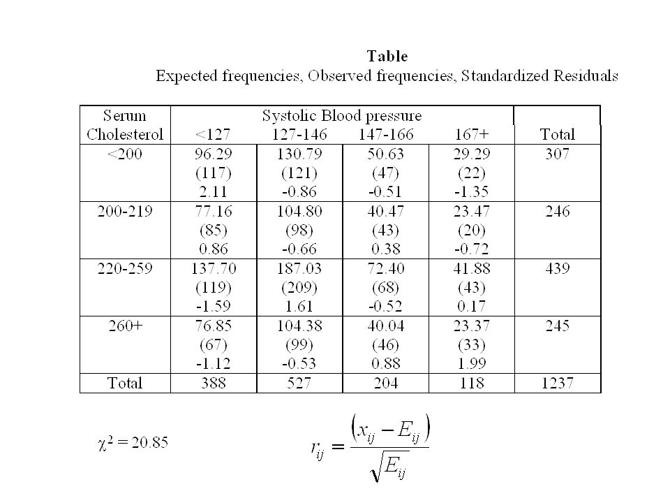
39. Example: studying the relationship between Systolic Blood pressure and Serum Cholesterol In this example we are interested in whether Systolic Blood pressure and Serum Cholesterol are related or whether they are independent. Both were measured for a sample of n = 1237 cases

40. Serum Cholesterol Systolic Blood pressure <127127-146147-166167+ Total < 200 1171214722307 200-219 85984320246 220-259 1152096843439 260+ 67994633245 Total3885272041181237 Observed frequencies

41. Serum Cholesterol Systolic Blood pressure <127127-146147-166167+ Total < 200 96.29130.7950.6329.29307 200-219 77.16104.840.4723.47246 220-259 137.70187.0372.4041.88439 260+ 76.85104.3840.0423.37245 Total3885272041181237 Expected frequencies In the case of independence the distribution across a row is the same for each row The distribution down a column is the same for each column

43. Standardized residuals The  2 statistic

44. Example This comes from the drug use data. The two variables are: 1. Role (C) and 2.Antidepressant Use (R) measured for a sample of n = 33,957 subjects.

45. Two-way Frequency Table Percentage antidepressant use vs Role

47. Calculation of  2 The Raw data Expected frequencies

48. The Residuals The calculation of  2

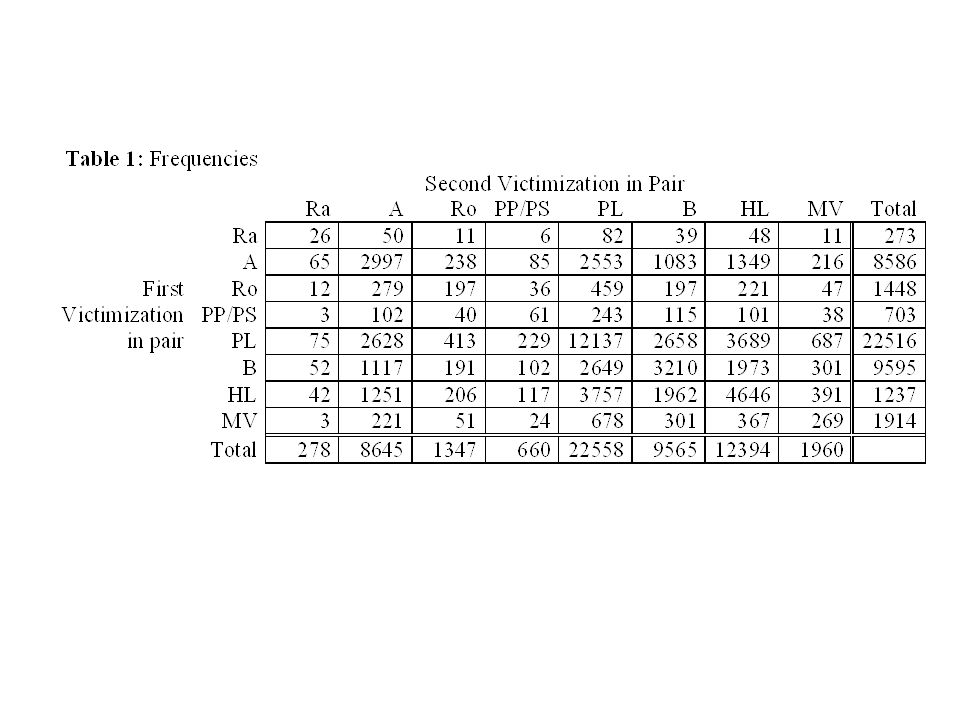
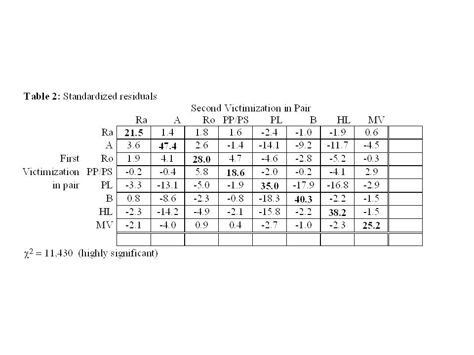
49. Example In this example n = 57407 individuals who had been victimized twice by crimes Rows = crime of first vicitmization Cols = crimes of second victimization

52. Next Topic: Brief introduction to Statistical Packages