Download presentation
Presentation is loading. Please wait.

1
MULTI-DISCIPLINARY INVERSE DESIGN George S. Dulikravich Dept. of Mechanical and Aerospace Eng. The University of Texas at Arlington gsd@mae.uta.edu

2
Professor Dulikravich has authored and co-authored over 250 technical publications in the diverse fields involving computational and analytical fluid mechanics, subsonic, transonic and hypersonic aerodynamics, theoretical and computational electro-magneto-hydrodynamics, conjugate heat transfer including solidification, computational cryobiology, acceleration of iterative algorithms, computational grid generation, and multi- disciplinary aero-thermo-structural inverse problems, design, and constrained optimization in turbomachinery. He is the founder and Editor-in-Chief of the international journal on Inverse Problems in Engineering and an Associate Editor of three additional journals. He is also the founder, chairman and editor of the sequence of International Conferences on Inverse Design Concepts and Optimization in Engineering Sciences (ICIDES). Professor Dulikravich is a Fellow of the ASME, an Associate Fellow of the AIAA, and a member of the AAM.
. Professor Dulikravich is a Fellow of the ASME, an Associate Fellow of the AIAA, and a member of the AAM..")
3
Multi-Disciplinary Inverse Problems Engineering field problems are defined (Kubo, 1993) by the governing partial differential or integral equation(s), shape(s) and size(s) of the domain(s), boundary and initial conditions, material properties of the media contained in the field, and by internal sources and external forces or inputs. If all of this information is known, the field problem is of an analysis (or direct) type and generally considered as well posed and solvable. If any of this information is unknown or unavailable, the field problem becomes an indirect (or inverse) problem and is generally considered to be ill posed and unsolvable. Specifically, inverse problems can be classified as: 1. Shape determination inverse problems, 2. Boundary/initial value determination inverse problems, 3. Sources and forces determination inverse problems, 4. Material properties determination inverse problems, and 5. Governing equation(s) determination inverse problems. The inverse problems are solvable if additional information is provided and if appropriate numerical algorithms are used.
 type and generally considered as well posed and solvable. If any of this information is unknown or unavailable, the field problem becomes an indirect (or inverse) problem and is generally considered to be ill posed and unsolvable. Specifically, inverse problems can be classified as: 1. Shape determination inverse problems, 2. Boundary/initial value determination inverse problems, 3. Sources and forces determination inverse problems, 4. Material properties determination inverse problems, and 5. Governing equation(s) determination inverse problems. The inverse problems are solvable if additional information is provided and if appropriate numerical algorithms are used..")
4
[H]{ }=[G]{q}+{P}
![[H]{ }=[G]{q}+{P}](http://images.slideplayer.com/34/8371450/slides/slide_4.jpg "[H]{ }=[G]{q}+{P}")
5
Inverse Determination of Thermal and Elasticity Boundary Conditions Mesh for multiply-connected domain

6
Inverse Detection of Unknown Boundary Conditions with FEM (Temperature Field) ForwardInverse Temperature
 ForwardInverse Temperature")
7
Inverse Detection of Unknown Boundary Conditions with FEM (Principal Stress Distribution) ForwardInverse Principle Stress
 ForwardInverse Principle Stress")
8
Inverse Heat Conduction Using BEM Convective Boundary Condition on a Rectangular Plate

9
Inverse determination of temperature on the bottom boundary: over-specified remaining three sides

10
Heat Conduction Using BEM Circular Disk with Circular Hole and Heat Generation

11
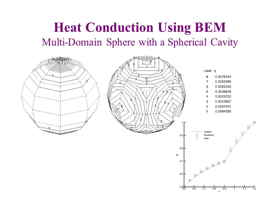
Heat Conduction Using BEM Multi-Domain Sphere with a Spherical Cavity

18
Inverse Electrocardiography Inverse electrocardiography uses multiple measurements taken on the chest surface to calculate the electrical activity throughout the heart This would allow physicians to accurately detect the origin of electrical anomalies Accurate location of anomalies allows the use of non-invasive treatment techniques

19
Forward Problem Results (continued) Analytic Potential Distribution, 23 dipoles Computed Potential Distribution, 23 dipoles
 Analytic Potential Distribution, 23 dipoles Computed Potential Distribution, 23 dipoles")
20
Forward Problem Results (continued) Analytic Potential Distribution, 23 dipoles Computed Potential Distribution, 23 dipoles
 Analytic Potential Distribution, 23 dipoles Computed Potential Distribution, 23 dipoles")
21
Inverse Problem Results (continued) Analytic Potential Distribution, 23 dipoles Computed Potential Distribution, 23 dipoles
 Analytic Potential Distribution, 23 dipoles Computed Potential Distribution, 23 dipoles")
22
Inverse Problem Results (continued) Relative Error Distribution, 23 dipoles
 Relative Error Distribution, 23 dipoles")
23
AERODYNAMIC SHAPE INVERSE DESIGN Develop a method that · can be applied in 3-D, · accepts any flow-field analysis code by calling it as a subroutine, · does not require flow-field analysis code modifications, · converges fast.

24
Full airplane aerodynamic shape inverse design using optimization as a tool

25
Inverse Shape Design Using Elastic Membrane Concept ( 2D & 3D movies) Model surface of an aerodynamic body as a membrane that deforms under aerodynamic loads until it achieves a desired surface pressure distribution.
 Model surface of an aerodynamic body as a membrane that deforms under aerodynamic loads until it achieves a desired surface pressure distribution.")
29
INVERSE DETERMINATION OF TEMPERATURE- DEPENDENT THERMAL CONDUCTIVITY USING STEADY SURFACE DATA ON ARBITRARY OBJECTS

30
Variation of the thermal conductivity versus temperature for various amounts of input error in boundary temperature (a) = 0.0 o C, (b) = 0.1 o C, (c) = 1.0 o C, and (d) = 5.0 o C.
 = 0.0 o C, (b) = 0.1 o C, (c) = 1.0 o C, and (d) = 5.0 o C.")
31
Predicted temperature-dependence of thermal conductivity when errors were added to the heat fluxes compared to the actual linear variation of k(T).
.")
32
Variation of the thermal conductivity versus temperature for various levels of input error in temperature, (a): = 0.0 o C, (b): = 0.5 o C, (c): = 1.0 o C, and (d): = 5.0 o C. The BEM results are compared to the actual arctangent conductivity versus temperature function

33
Variation of thermal conductivity versus temperature predicted with the beta-spline basis functions and with the integrated beta-spline basis functions. The inverse BEM results are compared to the actual arctangent conductivity versus temperature function

34
Inverse determination of the thermal conductivity of copper in the cryogenic range. The best inverse results are shown with various levels of input error: a) = 0.0 K, b) = 0.1 K, and c) = 1.0 K).
 = 0.0 K, b) = 0.1 K, and c) = 1.0 K)..")
35
Inverse prediction of thermal conductivity variation of an arbitrarily shaped specimen made of copper.

36
INFLUENCE OF BOUNDARY CONDITIONS ON MOISTURE DIFFUSIVITY ESTIMATION BY TEMPERATURE RESPONSE OF A DRYING BODY

37
The estimation methodology used is based on minimization of the ordinary least square norm. Here, Y T = [Y 1,Y 2, …,Y imax ] is the vector of measured temperatures and T T = [T 1 (P), T 2 (P), … T imax (P)] is the vector of estimated temperatures at time t i (i = 1, 2, …, imax), while P T = [P 1,P 2, … P N ] is the vector of unknown parameters, imax is the total number of measurements, and N is the total number of unknown parameters (imax N).
, T 2 (P), … T imax (P)] is the vector of estimated temperatures at time t i (i = 1, 2, …, imax), while P T = [P 1,P 2, … P N ] is the vector of unknown parameters, imax is the total number of measurements, and N is the total number of unknown parameters (imax N)..")
38
A version of Levenberg-Marquardt method was applied for the solution of the presented parameter estimation problem (Marquardt, 1963).
.")
39
Drying air conditions CaseDrying airTransfer coefficients 3 mm6 mmTa[0C]Ta[0C]V a [m/s]h[W/m 2 K]h D 10 2 [m/s] A1AA1 80 328.63.20 B1BB1 80 544.95.02 C1CC1 80 1083.19.29 A2AA2 120 329.33.55 B2BB2 120 545.95.56 C2CC2 120 1084.910.30
![Drying air conditions CaseDrying airTransfer coefficients 3 mm6 mmTa[0C]Ta[0C]V a [m/s]h[W/m 2 K]h D 10 2 [m/s] A1AA B1BB C1CC A2AA B2BB C2CC](http://images.slideplayer.com/34/8371450/slides/slide_39.jpg "Drying air conditions CaseDrying airTransfer coefficients 3 mm6 mmTa[0C]Ta[0C]V a [m/s]h[W/m 2 K]h D 10 2 [m/s] A1AA B1BB C1CC A2AA B2BB C2CC")
40
Sensitivity determinants

41
Sensitivity coefficients

42
Sensitivity coefficient (square symbols) and determinant (diamond symbols) for Case C2
 and determinant (diamond symbols) for Case C2")
43
Transient moisture content and temperature profiles

44
CONCLUSIONS & RECOMMENDATIONS - need for fast iterative solvers for sparse ill- conditioned matrices - need for better regularization algorithms - need for multi-disciplinary inverse problems solutions - need for combining inverse and optimization algorithms

Similar presentations


 St. Petersburg Polytechnical University Author:>")


 Applied to a High Pressure Gas Turbine Vane David Wasserman MEAE 6630 Conduction Heat Transfer Prof. Ernesto Gutierrez-Miravete.>")
