Transfer Learning Delasa Aghamirzaie, Abraham Lama Salomon

Name: Transfer Learning Delasa Aghamirzaie, Abraham Lama Salomon
Uploaded: 2017-07-21T14:00:06+00:00
Duration: PTM25S38
Channel: Marvin Allison
Description: Transfer Learning Delasa Aghamirzaie, Abraham Lama Salomon

Transfer Learning Delasa Aghamirzaie, Abraham Lama Salomon
Deep Learning for Perception 9/15/2015

Outline

slide credit Jason Yosinski
Convolutional Neural Networks: AlexNet Lion Successful training of a very large CNN on imagenet data to predict one of the thousand classes. We know these models are working labels Image Krizhevsky, Sutskever, Hinton — NIPS 2012 slide credit Jason Yosinski

Layer 1 Filter (Gabor and color blobs) Zeiler et al. arXiv 2013, ECCV 2014 Layer 2 Layer 5 Last Layer Nguyen et al. arXiv 2014 clear THAT they work, but not as clear WHY or HOW. WHAT’s going on in the middle? LET’S think about what we DO KNOW. It does not matter what dataset you use or what task you are training on, the first layer is always a gabor filter. To find patches of images that cause high activation: deconvulutional neural network Gabor filter: linear filters used for edge detection with similar orientation representations to the human visual system slide credit Jason Yosinski

general ?? Main idea of this paper: Quantify the general to specific transition by using transfer learning. Lion At the beginning layers we learn features that are general. At the last layers, we learn features that are specific to the target task. The question is how this transition occurs. Quantify the transition using transfer learning. Specific to tasks, specific Layer number slide credit Jason Yosinski

Transfer Learning Overview
Defining transfer learning How it works Frozen weights Fine tuning Selffer Fine tuner Transfer Figure for demonstrating how backprop woks Task A Input A Layer n Transfer AnB: Frozen Weights Back-propagation Task B Input B Task B Back-propagation AnB+: Fine-tuning

ImageNet dataset A B 500 Classes 1000 Classes okapi slide credit Jason Yosinski Deng et al., 2009

A Images A Labels Train using Caffe framework (Jia et al.) slide credit Jason Yosinski 500 Classes

train using the Caffe A Images A Labels Train using Caffe framework (Jia et al.) slide credit Jason Yosinski 500 Classes

A Images A Labels Train using Caffe framework (Jia et al.) slide credit Jason Yosinski 500 Classes

baseA A Images baseB B Images slide credit Jason Yosinski

Each point is average accuracy over validation set. Variants because of different 500 classes. slide credit Jason Yosinski

A Images A Labels slide credit Jason Yosinski

B Images B Labels Hypothesis: if transferred features are specific to task A, performance drops. Otherwise the performance should be the same. slide credit Jason Yosinski

transfer AnB B Images B Labels baseB Compare to slide credit Jason Yosinski

FIRST layers generic for this A / B combination OVERALL drop by the end is not large! (MANY RELATED CATEGORIES) CURIOUS BUMP IN MIDDLE slide credit Jason Yosinski

B Images B Labels slide credit Jason Yosinski

selffer BnB B Images B Labels slide credit Jason Yosinski

When you chop half of the network, randomly initialize the rest of the network, keep the weights frozen, u have optimization issues. A so slide credit Jason Yosinski

Performance drops due to... Fragile co-adaptation Representation specificity Not previously shown slide credit Jason Yosinski

Not previously shown slide credit Jason Yosinski

Transfer + fine-tuning improves generalization Not previously shown slide credit Jason Yosinski

ImageNet has many related categories... Dataset A: random Dataset B: random gecko garbage truck toucan fire truck radiator binoculars baseball lion panther bookshop rabbit gorilla slide credit Jason Yosinski

ImageNet has many related categories... Dataset A: man-made Dataset B: natural garbage truck gorilla fire truck gecko radiator toucan baseball rabbit binoculars panther bookshop lion slide credit Jason Yosinski

Similar A/B slide credit Jason Yosinski

Similar A/B Dissimilar A/B slide credit Jason Yosinski

Similar A/B Random (Jarret et al. 2009) Dissimilar A/B slide credit Jason Yosinski

Conclusions Measure general to specific transition layer by layer
fine-tuning helps co-adaptation specificity Measure general to specific transition layer by layer Transferability governed by: lost co-adaptations specificity difference between base and target dataset Fine-tuning helps even on large target dataset In top-5 accuracy you give yourself credit for having the right answer if the right answer appears in your top five guesses.

DeCAF: A Deep Convolutional Activation Feature
for Generic Visual Recognition Jeff Donahue, Yangqing Jia, Oriol Vinyals, Judy Hoffman, Ning Zhang, Eric Tzeng and Trevor Darrell Yangqing Jia, author of Caffe and its precursor DeCAF.

Problem: performance with conventional visual representations had reached a plateau. Solution: discover effective representations that capture salient semantics for a given task. can deep architectures do this?

Why Deep Models: deep architectures should be able to capture salient aspects of a given domain [Krizhevsky NIPS 2012][Singh ECCV 2012]. perform better than traditional hand-engineered representations [Le CVPR 2011] Had been applied to large-scale visual recognition tasks However: with limited training data, fully-supervised deep architectures generally overfit many visual recognition challenges have tasks with few training examples

Approach: Train a Deep convolutional model in a fully supervised setting using Krizhevsky method and ImageNet database. [Krizhevsky NIPS 2012]. Extract various features from the network Evaluate the efficacy of these features on generic vision tasks Questions: Do features extracted from the CNN generalize the other datasets ? How does performance vary with network depth? How does performance vary with network architecture?

Adopted Network: Deep CNN architecture proposed by Krizhevsky [Krizhevsky NIPS 2012]. 5 convolutional layers (with pooling and ReLU) 3 fully-connected layers won ImageNet Large Scale Visual recognition Challenge 2012 top-1 validation error rate of 40.7% follow architecture and training protocol with two differences input 256 x 256 images rather than 224 x 224 images no data augmentation trick

Qualitatively and Quantitatively Feedback:
Comparison with GIST features [Oliva & Torralba, 2001] and LLC features [Wang at al., 2010] Use of t-SNE algorithm [van der Maaten & Hilton, 2008] Use of ILSVRC-2012 validation set to avoid overfitting (150,000 photographs) Use of SUN-397 dataset to evaluate how dataset bias affects results

Feature Generalization and Visualization
T-SNE Algorithm t-SNE feature visualizations on the ILSVRC-2012 validation set LLC Features GIST Features DeCAF We visualize features in the following way: we run the t- SNE algorithm (van der Maaten & Hinton, 2008) to find a 2-dimensional embedding of the high- imensional feature space, and plot them as points colored depending on their semantic category in a particular hierarchy. LLC FEATURES

LLC FEATURES DeCAF1 FEATURES This is compatible with common deep learning knowledge that the first layers learn “low-level” features, whereas the latter layers learn semantic or “highlevel” features. Furthermore, other features such as GIST or LLC fail to capture the semantic difference in the image GIST FEATURES DeCAF6 FEATURES

DeCAF6 features trained on ILSVRC-2012 generalized to SUN-397 when considering semantic groupings of labels SUN-397: Large-scale scene recognition from abbey to zoo. (899 categories and 130,519 images)

Computational Time Break-down of the computation time analyzed using the decaf framework. The convolution and fully-connected layers take most of the time to run, which is understandable as they involve large matrix-matrix multiplications6.

Experimental Comparison Feedback
Not evaluation of features from any earlier layers in the CNN do not contain rich semantic representation Results on multiple datasets to evaluate the strength of DeCAF for basic object recognition (Caltech-101) domain adaptation (Office) fine-grained recognition (Caltech-UCSD) scene recognition (SUN-397)

Experiments: Object Recognition
Caltech-101 Compared also with the two-layers convolutional network of Jarret et al (2009)

Experiments: Domain Adaptation
Office dataset (Saenko et al., 2010), which has 3 domains: Amazon: images taken from amazon.com Webcam and Dslr: images taken in office environment using a webcam or SLR camera

Experiments: Domain Adaptation
DeCAF robust to resolution changes DeCAF provides better category clustering than SURF DeCAF clusters same category instances across domains The dataset contains three domains: Amazon, which consists of product images taken from amazon.com; and Webcam and Dslr, which consists of images taken in an office environment using a webcam or digital SLR camera, respectively. DeCAF6 FEATURES GIST FEATURES

Experiments: Subcategory Recognition
Fine grained recognition involves recognizing subclasses of the same object class such as different bird species, dog breeds, flower types, etc. Caltech-UCSD birds dataset First adopt ImageNet-like pipeline, DeCAF6 and a multi-class logistic regression Second adopt deformable part descriptors (DPD) method [Zhang et al., 2013]

Experiments: Scene Recognition
Goal: classify the scene of the entire image SUN-397 large-scale scene recognition database Outperforms Xiao ed al. (2010), the current state-of-the-art method DeCAF demonstrate the ability to generalize to other tasks - representational power as compared to traditional hand-engineered features

Are the features extracted by a deep network could be exploited for a wide variety of vision tasks?
CNN representation replaces pipelines of service-oriented architecture (s.o.a) methods and achieve better results.

OverFeat: publicly available trained CNN, with a structure that follows Krizhevsky et al. Trained for image classification of ImageNet ILSVRC 2013 (1.2 million images, 1000 categories). The features extracted from the OverFeat network were used as a generic image representation The CNN features used are trained only using ImageNet data, while the simple classifiers are trained using images specific to the task’s dataset.

Experimental Comparison Feedback
Results on multiple different recognition tasks: visual classification (Pascal VOC 2007, MIT-67 ) fine-grained recognition (Caltech-UCSD, Oxford 102) attribute detection (UIUC 64, H3D dataset) visual image retrieval (Oxford5k, Paris6k, Sculptures6k, Holidays and Ukbench)

Visual Classification
The feature vector is L2 normalized to unit length for all the experiments. The 4096 dimensional feature vector was used in combination with a Support Vector Machine (SVM) to solve different classification tasks (CNN-SVM). The training set was augmented by adding cropped and rotated samples (CNNaug+ SVM).

Databases: Pascal VOC for object image classification. Pascal VOC 2007 contains images of 20 classes including animals, handmade and natural objects. MIT-67 indoor scenes for scene recognition. The MIT scenes dataset has 15620 images of 67 indoor scene classes. In contrast to object detection, object image classification requires no localization of the objects.

Pascal VOC 2007 Image Classification Results compared to other methods which also use training data outside VOC. The CNN representation is not tuned for the Pascal VOC dataset

Evolution of the mean image classification AP (average precision) over PASCAL VOC 2007 classes as we use a deeper representation from the OverFeat CNN trained on the ILSVRC dataset. Intuitively one could reason that the learnt weights for the deeper layers could become more specific to the images of the training dataset and the task it is trained for. We observed the same trend in the individual class plots. The subtle drops in the mid layers (e.g. 4, 8, etc.) is due to the “ReLU” layer which half-rectifies the signals. Although this will help the non-linearity of the trained model in the CNN, it does not help if immediately used for classification.

Confusion matrix for the MIT-67 indoor dataset. Some of the off-diagonal confused classes have been annotated, these particular cases could be hard even for a human to distinguish.

Results of MIT 67 Scene Classification Using a CNN off-the-shelf representation with linear SVMs training significantly outperforms a majority of the baselines. The performance is measured by the average classification accuracy of different classes (mean of the confusion matrix diagonal).

Fine Grained Recognition
Results on CUB Bird dataset.

Fine Grained Recognition
Results on the Oxford 102 Flowers dataset

Attribute Detection An attribute is a semantic or abstract quality which different instances/categories share. Databases: UIUC 64 object attributes dataset. There are 3 categories of attributes in this dataset: shape (e.g. is 2D boxy) part (e.g. has head) material (e.g. is furry). H3D dataset which defines 9 attributes for a subset of the person images from Pascal VOC The attributes range from “has glasses” to “is male”.

Attribute Detection UIUC 64 object attribute dataset results
H3D Human Attributes dataset results.

Visual Image Retrieval
The result of object retrieval on 5 datasets

Image Representation:
Shallow Features: handcrafted classical representations. Improved Fisher Vector (IFV). Deep Features: CNN based representations.

Comparison: ConvNet based feature representations with different pre-trained network architectures and different learning heuristics.

CNN-F Network (Fast Architecture)
Similar to Krizhevsky et al. (ILSVRC-2012 winner) Fast processing is ensured by the 4 pixel stride in the first convolutional layer

CNN-M Network (Medium Architecture)
Similar to Zeiler & Fergus (ILSVRC-2013 winner) Smaller receptive window size + stride in conv1

CNN-S Network (Slow Architecture)
Similar to Overfeat ‘accurate’ network (ICLR 2014) Smaller stride in in conv2

VGG Very Deep Network Simonyan & Zisserman (ICLR 2015) Smaller receptive window size + stride, and deeper

Data Augmentation: Given pre-trained ConvNet, augmentation applied at test time

Data Augmentation:

TN-CLS TN-RNK Fine-tuning: TN-CLS – classification loss
TN-RNK – ranking loss

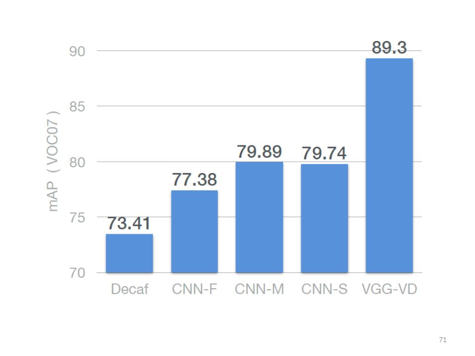
Evolution of Performance on PASCAL VOC-2007 over the recent years

Key points: We can learn features to perform semantic visual discrimination tasks using simple linear classifiers CNN features tend to cluster images into interesting semantic categories on which the network was never explicitly trained. Performance improves across a spectrum of visual recognition tasks. Data augmentation helps a lot, both for deep and shallow features. Fine tuning makes a difference, and should use ranking loss where appropriate.

CloudCV CloudCV DeCAF Server

Questions

Transfer Learning Delasa Aghamirzaie, Abraham Lama Salomon

Similar presentations

Presentation on theme: "Transfer Learning Delasa Aghamirzaie, Abraham Lama Salomon"— Presentation transcript:

Similar presentations

About project

Feedback

Log in

Auth with social network:

Transfer Learning Delasa Aghamirzaie, Abraham Lama Salomon

Similar presentations

Presentation on theme: "Transfer Learning Delasa Aghamirzaie, Abraham Lama Salomon"— Presentation transcript:

Similar presentations

About project

Feedback